USSR STATE COMMITTEE FOR
SUPERVISION OVER SAFE WORK PRACTICES
IN THE NUCLEAR POWER INDUSTRY
(USSR GOSATOMENERGONADZOR)
RULES AND REGULATIONS IN THE
NUCLEAR POWER INDUSTRY
|
Approved
by
The USSR State Committee for Atomic Energy Use
|
Approved by
The USSR State Committee for Supervision over Safe Work Practices in the Nuclear Power Industry (USSR Gosatomenergonadzor)
|
RULES OF EQUIPMENT AND
PIPELINES STRENGTH CALCULATION OF
NUCLEAR POWER PLANTS
PNAE G-7-002-86
Mandatory for
all ministries, administrations, organizations and enterprises
designing, constructing, manufacturing and operating nuclear
power plants, heating plants, experimental and research nuclear reactors
and installations controlled by the USSR Gosatomenergonadzor
Effective from July 1, 1987 with amendments

MOSCOW ENERGOATOMIZDAT 1989
The
regulations contain the main part and recommended appendices. The main
(mandatory) part contains: calculation for selection of basic dimensions;
calculation of static strength, resistance, cyclic strength, brittle fracture
resistance, long-term static strength, long-term cyclic strength, progressive
form change, seismic impacts, vibration strength; methods for determining
mechanical properties and tests to determine the strength characteristics.
CONTENTS
|
1. General
1.1. Scope of the
Regulations
1.2. Principles
Underlying the Regulations
2. Basic Definitions
3. Permissible
Stresses and Strength and Stability Conditions
4. Calculation for
Selection of Basic Dimensions
4.1. General
4.2. Determination of
Wall Thickness of the Components of Equipment and Pipelines
4.3. Strength
Reduction Coefficients and Strengthening of Holes
4.4. Flanges, Pressure
Rings, and Fasteners
5. Checking
Calculation
5.1. General
5.2. Classification of
Stresses
5.3. Stress
Calculation Procedure
5.4. Calculation for
Static Strength
5.5. Calculation for
Stability
5.6. Calculation for
Cyclic Strength
5.7. Calculation for
Long-Term Cyclic Strength
5.8. Calculation for
Resistance to Brittle Fracture
Appendix 1 Physical
and Mechanical Properties of Structural Materials
Appendix 2 Methods for
Determining Mechanical Properties of Structural Materials
1. Additional Concepts
and Definitions
2. Tension Test
Methods
3. Creep Test Methods
4. Long-Term Strength
Test Methods
5. Method for
Determining Critical Brittle Temperature
6. Procedure for
Determining Critical Brittle Temperature Shift due to Thermal Ageing
7. Procedure for
Determining Critical Brittle Temperature Shift due to Fatigue Damage
Accumulation
8. Procedure for
Determining Critical Brittle Temperature Shift due to Effects of
Exposure and Radiation Embrittlement Coefficient
9. Fatigue Test
Methods
10. Methods for
Process Tests of Metals
11. Welded Joints.
Methods for Determining Mechanical Properties
Appendix 3 Unified
Methods for Design and Experimental Determination of Stresses, Deformations,
Displacements, and Forces
1. Basic Provisions
2. Calculation of
Stresses, Displacements and Forces in Axisymmetric Structures of Thin-Walled
Shells, Plates and Rings under Axisymmetric Loading
3. Calculation of
Stresses and Displacements in Axisymmetric Thick-Walled Components of
Structures
4. Calculation of
Local Stresses in Components of Structures
5. Experimental
Determination of Stress and Displacement Deformations
Appendix 4 Calculation
of Components of Structures for Progressive Form Change
1. General
2. Definitions. Rated
Stresses
3. Limit Stresses
4. Additional
Conventional Symbols
5. Sequence of
Calculation for Progressive Form Change in the Absence of Irradiation Growth
6. Example of
Calculation of Cylindrical Shell
7. Adaptability
Diagrams for Some Standard Design Models
8. Method for
Determining the Value of Irreversible Form Change under Neutron Exposure
Conditions
9. Example of
Calculating Upper and Lower Estimations of Limit Cycle Parameters
Appendix 5 Calculation
of Standard Assemblies of Parts and Structures
1. Basic Provisions
2. Pipelines
3. Detachable
Connections of Vessels
Appendix 6
Characteristics of Long-Term Strength, Ductility and Creep of Structural
Materials
1. Basic Concepts and Symbols
2. General
3. Extrapolation
Method for Long-Term Strength
4. Extrapolation
Method for Conditional Limits of Creep
5. Extrapolation
Method for Conditional Limits of Stress Rupture Ductility
Appendix 7 Calculation
for Long-Term Cyclic Strength
Appendix 8 Design and
Experimental Methods for Assessment of Vibration Strength of Standard
Components of Structures
1. General
2. Calculation of
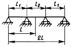
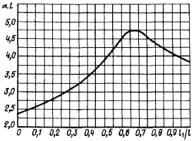
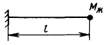
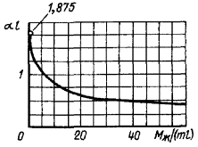
Natural Oscillation Frequency of Bar Systems
3. Calculation of
Natural Oscillation Frequency of Isotropic Rectangular Plates
4. Calculation of
Natural Oscillation Frequency of Shallow Rectangular Shell
5. Experimental
Methods for Vibration Research
6. Recommended Methods
for Assessment of Vibration Strength of Components of Structures
Appendix 9 Calculation
for Seismic Impacts
1. Generalized
Response Spectra
2. Unified Methods for
Calculating Equipment and Pipelines for Strength from Seismic Impacts
3. Procedures for
Calculating Pipelines for Seismic Impacts
Appendix 10
Selection of Basic
Sizes of Flanges, Pressure Rings, and Fasteners
1. Conventional
Symbols
2. Selection of
Sealing
3. Determination of
Forces in Pins
4. Determination of
Sizes of Flange Connections
5. Moments of
Deflection
6. Flange Face Height
Appendix 11
Recommendations for Determining the Process Increase to the Elbow Wall
Thickness
Appendix 12 Simplified
Cyclic Strength Calculation
1. Basic Provisions
2. Determination of
Change of Temperatures, Stresses, and Number of Operating Cycles
3. Verification of
Cyclic Strength
|
Basic
Conventional Symbols
Da – nominal
outer diameter of cylindrical part of a body, head or pipeline, mm
D – nominal
inner diameter of cylindrical part of a body, lid, head or pipeline, mm
Dm – mean
diameter of cylindrical part of a body, lid, head or pipeline, mm
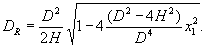
DR – design
diameter of round flat head or lid, mm
Dn – outer
diameter of a cover plate, mm
Rs – radius of
elbow axis, mm
R – inner
radius of convex head, mm
d – hole
diameter, mm
dR – design
hole diameter, mm
d0 – maximum
permissible diameter of non-strengthened hole, mm
dac – outer
diameter of a nozzle, mm
d01, d02
– major and minor axis of oval hole, mm
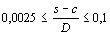
s – nominal
wall thickness, mm
sR – design
wall thickness, mm
s0 – minimum
design wall thickness, mm
sf – actual
wall thickness, mm
sc – nozzle
wall thickness, mm
sn – cover plate
thickness, mm
c – total
increase in wall thickness, mm
c11 – increase
in wall thickness equal to negative allowance, mm
c12 –
increase in wall thickness compensating for possible thinning of the
semi-finished product during manufacturing, mm
c2 – increase
in wall thickness considering wall thinning due to all types of corrosion
during service life of a product, mm
H – height of
convex part of a head to the inner surface, mm
Hm – height of
convex part of a head to the middle surface, mm
As – sectional
area of a component of structure, mm
L – design
length of shell, mm
Lkr – critical
length of shell, mm
φ – design strength
reduction coefficient
φd –
coefficient of strength reduction of shells or heads with a non-strengthened
hole
φc –
coefficient of strength reduction of shells or heads with a strengthened hole
φw –
coefficient of strength reduction of a weld seam
φ0 – minimum
permissible strength reduction coefficient
p – design
pressure, MPa (kgf/mm2)
pa – external
pressure, MPa (kgf/mm2)
pkr – critical
pressure, MPa (kgf/mm2)
F –
compressive force, N (kgf)
[pa] – permissible
external pressure, MPa (kgf/mm2)
[F] – permissible
compressive force, N (kgf)
T – design
temperature, K (°C)
Tt –
temperature above which the parameters of long-term strength, ductility, and
creep shall be taken into account, K (°C)
Tk – critical
brittle temperature, K (°C)
Tk0 – material
critical brittle temperature in the initial state, K (°C)
Th – hydraulic
(pneumatic) test temperature, K (°C)
∆TT – critical
brittle temperature shift due to temperature ageing, K (°C)
∆TN – critical
brittle temperature shift due to cyclic damaging, K (°C)
∆TF – critical
brittle temperature shift due to neutron exposure, K (°C)
σ - stresses, MPa
(kgf/mm2)
σm –
general membrane stresses, MPa (kgf/mm2)
σmL –
local membrane stresses, MPa (kgf/mm)
σb –
general bending stresses, MPa (kgf/mm2)
σbL –
local bending stresses, MPa (kgf/mm2)
σT –
general temperature stresses, MPa (kgf/mm2)
σTL –
local temperature stresses, MPa (kgf/mm2)
σc –
compensation stresses, MPa (kgf/mm2)
σcm –
tension or compression compensation stresses, MPa (kgf/mm2)
σcb –
bending compensation stresses, MPa (kgf/mm2)
τcs –
torsional compensation stresses, MPa (kgf/mm2)
σmw –
mean tension stresses over the cross-section of a bolt or pin, MPa (kgf/mm2)
τsw –
torsional stresses in bolts or pins, MPa (kgf/mm2)
σ1, σ2,
σ3 – main stresses, MPa (kgf/mm2)
σkr –
critical compression stress, MPa (kgf/mm2)
σc –
compression stress, MPa (kgf/mm2)
(σ)1, (σ)2,
(σ)3w, (σ)4w, (σs)1,
(σs)2, (σs)3w,
(σs)4w – groups of reduction of stresses,
MPa (kgf/mm2)
(σ)RV
– range of reduced stresses in equipment components, MPa (kgf/mm2)
(σ)RK
– range of reduced stresses in pipeline components, MPa (kgf/mm2)
σi, σj,
σk – stresses at main sites i, j, k, MPa
(kgf/mm2)
(σ)ij,
(σ)jk, (σ)ik, (σ) – reduced stresses
without concentration, MPa (kgf/mm2)
|
(σL)ij,
(σL)jk, (σL)ik,
(σL)
|
 
|
– local reduced
stresses calculated with due regard to the theoretical stress concentration
coefficient, MPa (kgf/mm2)
|
|
(σF)ij,
(σF)jk, (σF)ik,
(σF)
|

|
– local conditional
elastic reduced stresses calculated with due regard to the conditional
elastic stress concentration coefficient, MPa (kgf/mm2)
|
σa –
stress amplitude without concentration, MPa (kgf/mm2)
σaF – local
stress amplitude with due regard to concentration, MPa (kgf/mm2)
(σa) –
reduced stress amplitude without concentration, MPa (kgf/mm2)
(σaF)
– amplitude of conditional elastic reduced stresses with due regard to the
concentration coefficient of conditional elastic stresses, MPa (kgf/mm2)
(σaF)V
– amplitude of reduced stresses in equipment components, MPa (kgf/mm2);
(σaF)K
– amplitude of reduced stresses in pipeline components, MPa (kgf/mm2)
(σaF)W
– amplitude of reduced stresses in bolts or pins, MPa (kgf/mm2)
(σaL)
– amplitude of reduced stresses with due regard to the theoretical
concentration coefficient, MPa (kgf/mm2)
(σF)max
– maximum reduced conditional elastic stress of a cycle with due regard to the
concentration coefficient of conditional elastic stresses, MPa (kgf/mm2)
<σa>
– vibration stress amplitude, MPa (kgf/mm2)
[σ] – nominal
permissible stress, MPa (kgf/mm2)
[σ]Th
– nominal permissible stress at hydrotest temperature, MPa (kgf/mm2)
[σc] –
permissible compression stress, MPa (kgf/mm2)
RTm – minimum
value of ultimate resistance at design temperature, MPa (kgf/mm2)
RTp0.2 – minimum
value of yield limit at design temperature, MPa (kgf/mm2)
RThp0.2 – minimum
value of yield limit at hydrotest temperature, MPa (kgf/mm2)
RT-1 – endurance
limit with symmetric axial tension-compression cycle at design temperature, MPa
(kgf/mm2)
t – time, h
RTmt – minimum
limit of long-term durability over time t at design temperature, MPa
(kgf/mm2)
RTct – creep
limit at design temperature at which deformation with due regard to the creep
reaches a predetermined value over time t, MPa (kgf/mm2)
RTpe –
proportionality limit at design temperature, MPa (kgf/mm2)
AT5 – relative
elongation of a fivefold sample at static fracture under tension at design
temperature, %
ZT – relative
reduction of a sample cross-section at static fracture under tension at design
temperature, %
αT –
coefficient of linear expansion at design temperature, 1/K (1/°C)
ET – modulus of
elasticity at design temperature, MPa (kgf/mm2)
μ – Poisson ratio
N – number of
load cycles of a component of structure in operation
N0 – number of
load cycles before cracking in structure
f0 – load rate,
Hz
f – rate of
high-frequency stress cycles, Hz
r – stress
cycle asymmetry coefficient
v –
deformation curve work-hardening exponent
Kσ –
theoretical stress concentration coefficient
K(σ) –
theoretical reduced stress concentration coefficient
Kef – effective
concentration coefficient of conditional elastic stresses
a –
accumulated fatigue damage
e –
deformation, %
Fn – transfer
of neutrons with energy of more than 0.5 MeV, n/m2
AF – radiation
embrittlement coefficient, K (°C)
KI – stress
intensity coefficient, MPa · m1/2 (kgf/mm3/2)
KIc – critical
stress intensity coefficient, MPa · m1/2 (kgf/mm3/2)
n0.2 – yield
limit safety coefficient
nm – ultimate
resistance safety coefficient
nmt – safety
coefficient for long-term strength limit
nσ – safety coefficient
for conditional local stresses in calculations for cyclic strength
nN – safety
coefficient for number of cycles in calculations for cyclic strength
SNR – State
Nuclear Regulations
NPI – Nuclear
Power Installation
NO – Normal
Operation
AO – Abnormal
Operation
–
NPI Rules –
"Rules of design and safe operation of equipment and pipelines of nuclear
power installations"
1. GENERAL
1.1. SCOPE OF THE REGULATIONS
1.1.1. These
"Rules of equipment and pipelines strength calculation of nuclear power
plants" (hereinafter referred to as the Rules) shall be applied to assess
the strength of equipment and pipelines of nuclear power plants (NPP), nuclear
heat generation plants (NHGP), nuclear heating plants (NHP), industrial heating
nuclear power plants (IHNPP) and installations with research or development
reactors with a coolant temperature of not exceeding 873 K (600 °C).
1.1.2. The Rules
apply to equipment and pipelines the design, manufacture, installation and
operation of which are carried out in full accordance with the NPI Rules.
1.1.3. The company
or organization which performed a relevant calculation shall be responsible for
the correct application of these regulations.
1.2. PRINCIPLES UNDERLYING THE
REGULATIONS
1.2.1. Calculation
methods adopted in the Regulations are based on the principles of assessment
for the following limiting states:
1) short-term
fracture (ductile and brittle);
2) creep
fracture under static load;
3) plastic
deformation across the entire part cross-section;
4)
accumulation of the maximum permissible creep deformation;
5) cyclic
accumulation of plastic deformations leading to unacceptable change of
dimensions or quasistatic fracture;
6) occurrence
of macrocracks under cyclic loads;
7) buckling
failure.
At
temperatures which do not cause creep of the material of structure, the
calculation for the specified limiting states is carried out using short-term
characteristics of time independent strength, ductility, and deformation
resistance of the material. An exception is the consideration of deformation
ageing and exposure when calculating the resistance to brittle fracture and to
occurrence of macrocracks under cyclic load. If equipment and pipelines are
operated at temperatures which cause creep of the material, the calculation is
carried out according to the specified limiting states using the
characteristics of short-term and long-term strength, short-term and long-term
ductility, and creep.
1.2.2. During the
design, strength of equipment and pipelines is calculated in two stages:
1) calculation
for selection of basic dimensions;
2) checking
calculation.
When assessing
the strength of equipment and pipelines, both the requirements of calculation
for selection of basic dimensions and the requirements of checking calculation
shall be fully satisfied.
1.2.3. When
performing calculations for selection of basic dimensions, the (internal and
external) pressure applied to equipment and pipelines is taken into account,
and for bolts and pins the tightening force is taken into account.
1.2.4. The main
characteristics of the materials used in determining the values of permissible
stresses are assumed to be temporary resistance, yield limit, rupture strength,
and creep limit (with limited deformation).
Permissible
stresses are set according to the specified characteristics by introducing
appropriate safety coefficients.
1.2.5. The basis
of the formulas used in calculation for selection of basic dimensions is the
method of limit loads corresponding to the following limit states: ductile
fracture, plastic deformation spread over the entire cross-section of equipment
or pipeline, loss of stability, and achievement of limit deformation.
1.2.6. After
calculation for selection of basic dimensions, a checking calculation is
carried out, including the necessary sections from the following list:
1) calculation
for static strength;
2) calculation
for stability;
3) calculation
for cyclic and long-term cyclic strength;
4) calculation
for resistance to brittle fracture;
5) calculation
for long-term static strength;
6) calculation
for progressive form change;
7) calculation
for seismic impacts;
8) calculation
for vibration strength.
Checking
calculation is based on the assessment of the strength according to the
permissible stresses, deformations, and stress intensity coefficients.
1.2.7. During
checking calculation all acting loads (including temperature impacts) are taken
into account and all modes of operation are considered.
1.2.8. Checking
calculation for static strength is carried out for determination of stresses at
all values of loads and temperatures in all design specified installation
operation modes and for comparison of the obtained values with those
permissible determined by the limit states indicated in subitems 1) and 3) of
item 1.2.1.
1.2.9. Checking
calculation for stability consists in determining permissible loads or
permissible operation life exceeding of which entails possibility of loss of
stability during loading by external pressure and compressive loads [see 7),
item 1.2.1].
1.2.10. Checking
calculation for strength at cyclic and long-term cyclic loading is carried out
based on the analysis of general and local stress to exclude the occurrence of
cracks [see 6), item 1.2.1].
Permissible
stress amplitudes are determined based on the characteristics of cyclic or
long-term cyclic strength with introduction of safety coefficients in
durability and stresses.
As a result of
calculation for strength under cyclic or long-term cyclic loading, the
permissible number of repetitions of operation modes for specified repeated
operational thermal and mechanical loads, temperatures, and operation life, or
permissible thermal and mechanical loads for a specified number of repetitions
of operation modes and operation life are determined.
1.2.11. Checking
calculation for resistance to brittle fracture is carried out based on
comparison of stress intensity coefficient with its critical value in order to
exclude the possibility of brittle fracture [see 1), item 1.2.1].
1.2.12. Long-term
static strength is calculated on the basis of a comparison of the effective
stresses in all modes allowed to prevent the fracture of equipment or pipelines
during long-term static loading [see 2) and 4), item 1.2.1].
Permissible
stresses are determined on the basis of the characteristics of resistance to
long-term static fracture, depending on the temperature and duration of
loading, with the introduction of stress safety coefficients.
As a result of
calculation, the permissible loads for specified modes and operation life or
permissible operation life for specified operation modes are determined.
1.2.13. Checking
calculation for progressive form change is carried out based on stress
condition analysis in order to exclude unacceptable residual changes in shape
and size [see 5), item 1.2.1].
Permissible
limit changes in shape and size as a result of process of accumulation of
irreversible plastic deformations are specified by the design (engineering)
organization in each particular case with due regard to intended use and
operation conditions of equipment and pipelines.
As a result of
calculation, the permissible loads for specified modes and operation life or
permissible operation life for specified operation modes are determined.
1.2.14. Checking
calculation of equipment and pipelines for seismic impacts is carried out with
due regard to combined action of operational and seismic loads.
Strength of
equipment and pipelines is assessed by permissible stresses, by permissible
displacements, by the criteria of cyclic strength and stability (the latter is
only for equipment).
1.2.15. Reduced
stresses to be compared with the permissible are determined in accordance with
the maximum shear stress theory with the exception of calculation of resistance
to brittle fracture when the reduced stresses are determined in accordance with
the maximum normal stress theory.
1.2.16.
Calculation of stresses, without taking into account concentration, is carried
out in the assumption of a linearly elastic behavior of the material, unless
otherwise indicated. In assessing the cyclic strength beyond the elastic limit,
a stress called conditional elastic stress is used. This stress is equal to the
product of the elastic-plastic deformation at the point under consideration and
the modulus of elasticity.
1.2.17. When performing
calculations for selection of basic dimensions, the increase of ultimate
strength and yield limit under irradiation is not taken into account. Decrease
in characteristics of ductility and resistance to brittle, fatigue, long-term
static fracture and creep due to the effect of exposure are taken into account
when carrying out appropriate calculations using these characteristics.
1.2.18. If
necessary, the checking calculation shall take into account the influence of
working media on the change in strength characteristics based on representative
experimental data.
2. BASIC DEFINITIONS
2.1. Design
pressure is the maximum overpressure in the equipment or pipeline used in the
calculation for selection of basic dimensions at which the operation of this
equipment or pipeline is allowed under the NO.
For safety
bodies of equipment and pipelines and for containments, the design pressure is
understood as the maximum overpressure which occurs in these bodies or
containments in case of depressurization of the protected equipment or
pipelines.
In case the
component of structure is simultaneously loaded with internal and external
pressures, the difference in these pressures, at which the design wall
thickness is maximal, is assumed as the design pressure.
2.2. Design temperature
is the temperature of the equipment or pipeline wall equal to the maximum
arithmetic mean value of temperature on its outer and inner surfaces in the
same cross-section under the NO (for the parts of nuclear reactor vessels, the
design temperature is determined with due regard to the internal heat release
as the arithmetic mean value of temperature distribution over the thickness of
the vessel wall).
2.3. Hydraulic
or pneumatic testing is test loading of equipment or pipelines with internal or
external pressure in order to verify their integrity after manufacture,
installation, certain lifecycle or repair.
The pressure
value of the hydraulic or pneumatic testing is determined in accordance with
the NPI Rules.
2.4. Tightening
of pins is loading of components of equipment or pipelines caused by tightening
of pins or bolts.
2.5. Start-up is
an operating mode, in the process of which external loads and temperatures vary
from initial values to values corresponding to the steady-state mode. During
start-up, the temperature and external loads may exceed the values
corresponding to the steady-state mode.
2.6.
Steady-state mode is an operating mode in which external loads and temperature
remain constant within ±5 % of nominal values.
2.7. Operation
of the emergency protection system is an operating mode in which, due to the
operation of the emergency protection system for reasons not related to AO and
occurrence of the emergencies, there is a change in temperatures and external
loads (towards both increasing and decreasing) from their values in the
steady-state mode, start-up, or shutdown, to the corresponding intermediate
values (in the particular case to atmospheric pressure and temperature).
2.8. Reactor
power change is an operating mode in which a transition occurs from one
steady-state mode of reactor operation to another (with the exemption of the
start-up and shutdown modes).
2.9. Shutdown is
an operating mode in which the temperature and external loads change from the
values of parameters of any operating mode to the initial values of parameters
during the start-up mode.
2.10. See the
definition of the NO mode in Appendix 1 to the NPI Rules.
2.11. See the
definition of the AO mode in Appendix 1 to the NPI Rules.
2.12. See the
definition of the emergency situation in Appendix 1 to the NPI Rules.
2.13. Cycle of
stress change is a change in stress from the initial value with the transition
through the maximum and minimum algebraic values to the initial one.
2.14. A
half-cycle of stress change is a change in stress from the maximum (minimum)
value to the minimum (maximum) value in the cycle under consideration.
2.15. Stress
range is the difference between the maximum and minimum stresses in the process
of one cycle of stress change.
2.16. Maximum
(minimum) cycle stress is the maximum (minimum) algebraic value of stresses for
one cycle of their change.
2.17. Life
cycle is the total time of steady-state and transient operating modes,
including AO and emergencies.
2.18. σm
- general membrane stresses caused by mechanical loads normal to the
cross-section in question distributed over the cross-section and equal to the
mean value of the stress in this cross-section.
2.19. σmL
– local membrane stresses caused by mechanical loads. Membrane stresses are
classified as local if the dimensions of the area within which the stresses
exceed 1.1 [σ] do not exceed  , and this area is
located no closer than
, and this area is
located no closer than  to another area where
the stresses exceed [σ].
to another area where
the stresses exceed [σ].
2.20. σb
– general bending stresses caused by action of pressure and mechanical loads
varying from the maximum positive value to the minimum negative value over the
entire cross-section and leading to bending of the vessel body or whole
pipeline.
2.21. σbL
– local bending stress caused by edge forces and momentum of mechanical loads.
2.22. σT
– general temperature stresses caused by non-equilibrium distribution of
temperature within the component volume or due to the difference in the
material linear expansion coefficients, in the limiting case leading to
unacceptable residual changes in shape and size of the structure.
2.23. σTL
– local temperature stresses caused by non-equilibrium distribution of
temperature within the component volume or due to the difference in the
material linear expansion coefficients, which can not cause unacceptable
residual changes in shape and size of the structure.
2.24. σc
– compensation stresses caused by congestion of free expansion of pipelines or
tubes. These stresses include stresses of tension or compression σcm,
bending σcb, torsion τcs.
2.25. σmw
– mean tension stresses over the cross-section of a bolt or pin caused by
mechanical loads (with or without due regard to tightening).
2.26. τsw
– torsional stresses in bolts and pins.
2.27. (σ)1
– group of reduced stresses, determined by the components of general membrane
stresses.
2.28. (σ)2
– group of reduced stresses, determined by the sums of the components of
general or local membrane and general bending stresses.
2.29. (σ)3w
– group of reduced stresses determined as a sum of mean tension stresses over
the cross-section of a bolt or pin caused by mechanical loads, including
tightening force, and by thermal impacts.
2.30. (σ)4w
– group of reduced stresses from mechanical and thermal impacts, including tightening
force determined by the components of tension, bending and torsional stresses
in bolts and pins.
2.31. (σs)1
– group of reduced stresses from mechanical loads and seismic impacts,
determined by the components of the general membrane stresses.
2.32. (σs)2
– group of reduced stresses from mechanical loads and seismic impacts,
determined by the components of membrane and general bending stresses.
2.33. (σs)mw
– group of reduced stresses, determined by sums of mean tension stresses over
the cross-section of a bolt or pin caused by mechanical loads and seismic
impacts.
2.34. (σs)4w
– group of reduced stresses from mechanical loads, thermal and seismic impacts
determined by the components of tension, bending and torsional stresses in
bolts or pins.
2.35. (σ)RV
– the maximum range of reduced stresses determined by the sums of the
components of general or local membrane stresses, general and local bending
stresses, general temperature stresses and compensation stresses in the
equipment.
2.36. (σ)RK
– the maximum range of reduced stresses determined by the sums of the
components of general or local membrane stresses, general and local bending
stresses, general temperature stresses and compensation stresses in the
pipelines.
2.37. (σaF)V
– amplitude of reduced stresses determined by the sums of the components of
general or local membrane stresses, general and local bending stresses, general
and local temperature stresses and compensation stresses with due regard to
stress concentration in the equipment.
2.38. (σaF)K
– amplitude of reduced stresses determined by the sums of the components of
general or local membrane stresses, general and local bending stresses, general
and local temperature stresses and compensation stresses with due regard to
stress concentration in the pipelines.
2.39. (σaF)W
– amplitude of reduced stresses determined by the sums of the components of
mean stresses over the cross-section of a bolt or pin caused by mechanical and
thermal impacts, bending stresses, torsional and temperature stresses with due
regard to stress concentration.
3.
PERMISSIBLE STRESSES AND STRENGTH AND STABILITY CONDITIONS
3.1. Nominal
permissible stresses are determined based on characteristics of material at the
design temperature.
3.2. Nominal permissible stresses for components
with design temperature equal to or lower than Tt are
calculated by the yield limit and temporary resistance.
For components
with design temperature above the temperature Tt, the nominal
permissible stresses are calculated by the yield limit, temporary resistance
and long-term strength.
3.3. Temperature
Tt is:
1) for
aluminum and titanium alloys 293 K (20 °C);
2) for
zirconium alloys 523 K (250 °C);
3) for carbon,
alloyed, silicon-manganese and high-chromium steels 623 K (350 °C);
4) for corrosion-resistant
steels of austenitic class, heat-resistant chrome-molybdenum-vanadium steels
and iron-nickel alloys 723 K (450 °C).
3.4. Nominal permissible stress for the
components of equipment and pipelines loaded with pressure is assumed to be the
minimum of the following values:
[σ] = min{RmT/nm;
RTp0.2/n0.2; RTmt/nmt}.
For components
of equipment and pipelines loaded with internal pressure,
nm = 2.6; n0.2
= 1.5; nmt = 1.5.
For components
of equipment and pipelines loaded with external pressure exceeding the internal
pressure,
nm = 2.6; n0.2
= 2; nmt = 2.
Final check
for stability and adjustment (if necessary) of the wall thicknesses, specified
as per this section, loaded with external pressure exceeding internal pressure
shall be carried out in accordance with Section 5.5.
3.5. Nominal
permissible stress in bolts or pins caused by pressure and tightening forces is
determined as
[σ]w
= RTp0.2/n0.2,
where n0.2
= 2.
Additionally,
in bolts and pins the temperature of which exceeds temperature Tt
as per Section 3.2, the nominal permissible stresses are set from
pressure as follows
[σ]wt
= RTmt/nTmt,
where nmt
= 3.
3.6. For bodies
of safety shells and containments, nominal permissible stresses are as follows
[σ]c
= min{RmT/nm; RTp0.2/n0.2},
where nm
= 1.85; n0.2 = 1.07.
3.7. When determining nominal permissible
stresses, the values of short- and long-term mechanical characteristics are assumed
in accordance with state or industry standards (GOST or OST) or technical
specifications (TU). In the absence of the necessary data in these documents,
one should be guided by the data given in Table P1.1 or P1.4.
3.8. At temperatures higher than Tt,
for a given limitation of the creep deformation, the components are calculated
by creep limit RTct. In the absence of information
on creep limits in GOST, OST, or TU, their determination by the isochronic
curves given for a number of materials in Appendix 6 is allowed.
Safety
coefficient of creep limit RTct is assumed to be
equal to one.
3.9. At
temperatures above Tt in those cases when the operation of
the structure includes two or more loading modes that differ in temperature or
load, the main dimensions shall satisfy the strength condition for accumulated
long-term static damage

where ti
is the duration of the i-th loading mode operation;
[t]i
is the permissible loading time corresponding to the limit of long-term
strength RTmt = nmtσi
(values of RTmt may be accepted as per Table 4
of Appendix 1); σi is the stress of the i-th
mode.
3.10. For steel
castings the required data for which are not available in state or industry
standards, in technical specifications or in Table 1 of Appendix 1,
yield limit and ultimate resistance values are assumed to be equal to: 85% of
the value given in Table 1 for the same rolled or forged steel grade if
the castings are subjected to 100% ultrasonic or radiographic control; 75% of
the above values for other castings.
3.11. Upon
contact of components of structures with reactor-grade sodium, calculations use
design values of mechanical characteristics, determined by multiplying the
values of RmT, RTp0.2,
RTmt, RTct by the
reduction coefficient ηt, depending on the type of material,
temperature and duration of operation.
When
performing a calculation for selection of basic dimensions and carrying out a
checking calculation for pearlite steels, the reduction coefficient is
determined by the formula
ηt
= 1 - 0.15hc/sR,
where hc
is the thickness of surface layer of steel, decarbonized by 30%.
The value of hc
is determined according to the specifications of the product. For steels grades
12Kh2M, 12Kh2M1FB, it is allowed to determine hc in the order
indicated below.
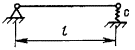
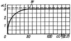
The upper
graph of Fig. 3.1 or 3.2 determines the point corresponding to
the specified design temperature T and operation time t, the
vertical from this point at the intersection with the curve of the lower graph
determines the point and the corresponding value of hc on the
vertical axis of this graph horizontally from the resulting point. Another way
is to calculate x according to formulas shown in Fig. 3.1 or 3.2
and to define the values of hc according to x, using
only the lower graph.
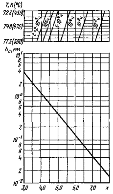
Fig. 3.1.
Diagram of 12Kh2M steel decarburization in liquid sodium, x = 7000/T
= lgt (T in K)
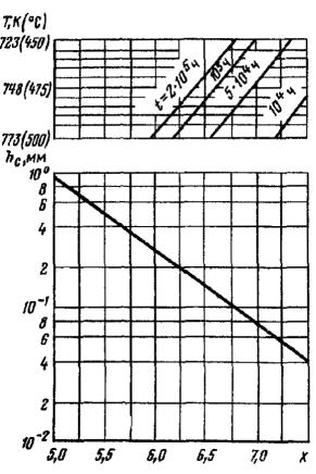
Fig. 3.2.
Diagram of 12Kh2M1FB steel decarburization in liquid sodium,
x = 8650/T = lgt (T in K)
When
performing a calculation for selection of basic dimensions and checking
calculation of parts with a wall thickness of more than 1 mm and time of
operation of not more than 2 · 105 h, the following is assumed:
for corrosion-resistant
austenitic steels with a nickel content of up to 15% at T ≤ 823 K (550
°C) ηt = 1 and at 823 K (550 °C) < T ≤ 973 K (700
°C) ηt = 0.9;
for iron-nickel alloys
at T ≤ 873 K (600 °C) ηt = 0.9 and at 873 K (600 °C)
< T ≤ 973 K (700 °C) ηt = 0.8.
4. CALCULATION FOR SELECTION OF BASIC
DIMENSIONS
4.1. GENERAL
4.1.1. When
performing a calculation for selection of basic dimensions, the design loads
are the design pressure and tightening forces for bolts and pins. When
calculating the flanges, pressure rings, and their fasteners, the hydrotest
pressure is taken into account.
4.1.2. When
determining the design wall thickness, the thickness of the anti-corrosion
deposited or clad protective layer is not taken into account.
4.1.3. The total
increase in the design thickness of the component of structure is defined as
c = c1
+ c2, where c1 = c11 + c12.
4.1.4. The
increase c2 takes into account the corrosive influence of
working medium on the material of the components of structure under operation
conditions. The values of this increase are determined by Table 4.1.
In cases not
listed in Table 4.1, the value of increase c2 is set
by the design (engineering) organization, with due regard to the corrosion rate
and operation time.
In case of
bilateral contact with a corrosive medium, the increase of c2
is assumed as total.
4.1.5. The
increase of c11 is determined according to the design
documentation and is assumed to be equal to the negative tolerance for the wall
thickness.
4.1.6. The
increase of c12 is a process one, designed to compensate for
the possible thinning of the semi-finished product during manufacture. The
value of this increase is set by the design (engineering) organization in
agreement with the manufacturer and shall be indicated in the detailed design.
The increase of c12 when calculating elbows is allowed to be
determined according to Appendix 11.
4.1.7. If
necessary, perform the calculation of the finished product using the actual
wall thickness of sf – c2.
Wall thickness
(sf – c2) for cylindrical and conical
components of structures is assumed to be equal to the mean value of four wall
thickness measurements at the ends of two mutually perpendicular diameters in
one section at a number of checked sections of at least one for every 2 m of
length. For round flat heads and lids, measurements are carried out in the
center and at four points along the circumference in two mutually perpendicular
directions, and the mean value is assumed to be equal to sf –
c2.
For elliptical
and hemispherical components of structures, measurements are performed in the
center and at four points along the ends of two largest mutually perpendicular
diameters, and the mean value is assumed to be equal to sf.
Table 4.1.
Value of increase c2
|
Material and its
welded joints
|
Operating
conditions of material in steady-state mode
|
Increase c2,
mm, for 30 years of operation
|
|
Corrosion-resistant
alloys of austenitic class
|
Water and steam-water
mixture, saturated steam up to 623 K (350 °C)
|
0.1
|
|
Pearlite steels
|
Water, 313 to 433 K
(40 to 160 °°C)
|
0.3
|
|
Water, 433 to 543 K
(160 to 270 °C)
|
1.2
|
|
Water, up to 623 K
(350 °C), pH = 8 ÷ 10
|
1.0
|
|
Saturated steam up to
573 K (300 °C)
|
1.0
|
|
Superheated steam
|
0.5
|
|
High chrome steels
|
Water and saturated
steam up to 558 K (285 °C)
|
0.1
|
|
Zirconium alloys
|
Water and steam-water
mixture up to 558 K (285 °C), reactor medium (mixture of helium with
nitrogen, up to 1% moisture by weight)
|
0.1
|
If the
component has local thinning that occurs during manufacture (stamping of heads,
pipe bending, etc.) or due to corrosion, then the actual wall thickness is set
depending on the location and size of the thinned section.
4.1.8. For
components not listed in Section 4, or if the limit of applicability of
the above formulas is violated, the selection of basic dimensions is carried
out according to the methods which shall be agreed with the organization
determined by the USSR Gosatomenergonadzor on case by case basis.
4.2. DETERMINATION OF WALL
THICKNESS OF THE COMPONENTS OF EQUIPMENT AND PIPELINES
4.2.1.
Cylindrical, conical shells of vessels and convex heads operating under
internal or external pressure.
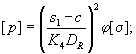
4.2.1.1. The design
wall thickness is determined by the formula
Values of
coefficients m1, m2, m3
and limits of applicability of the formulas are given in Table 4.2.
Table 4.2. Values
of coefficients m1, m2, m3
and limits of applicability of formulas
|
Value
|
Cylindrical
shell
(Fig. 4.1)
|
Conical
shell
(Fig. 4.2)
|
Elliptical
or torospheric head (Fig. 4.3)
|
Hemispherical
head
(Fig. 4.4)
|
|
m1
|
2
|
2
|
4
|
4
|
|
m2
|
1
|
cos α
|
1
|
1
|
|
m3
|
1
|
1
|
D/(2H)
|
1
|
|
Limits of
applicability
|

|
 α ≤
45°; α ≤
45°;
|

|
|
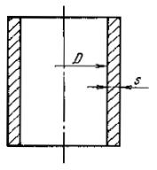
Fig. 4.1.
Cylindrical shell
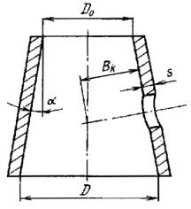
Fig. 4.2.
Conical shell
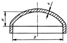
Fig. 4.3.
Elliptical or torospheric head
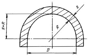
Fig. 4.4.
Hemispherical head
4.2.1.2. The assumed
nominal wall thickness shall satisfy the condition
s ≥ sR
+ c.
4.2.1.3. Permissible
pressure during design and after manufacture of vessels is determined by the
formulas:
during design

after manufacture
4.2.2. Cylindrical
headers, nozzles, pipes, and elbows.
4.2.2.1. The design
wall thickness of a cylindrical header, nozzle, and pipe is determined by the
formula

This formula
applies to (s - c)/Da ≤ 0.25.
4.2.2.2. The assumed
nominal wall thickness of a cylindrical manifold, nozzle, and pipe shall
satisfy the condition of item 4.2.1.2.
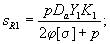
4.2.2.3. For
internal pressure elbows with an ratio of Rs/Da
≥ 1 (Fig. 4.5), the design wall thickness is determined by the formulas:
for the outside of the
elbow
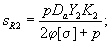
for the inside of the
elbow
for the middle part of
the elbow (in section A – A ± 15 ° from the neutral line of the
elbow)
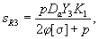
where K1,
K2, K3 are toroidal coefficients; Y1,
Y2, Y3 are shape coefficients.
4.2.2.4. Nominal
elbow wall thickness
s ≥ max{sR1,
sR2, sR3} + c.
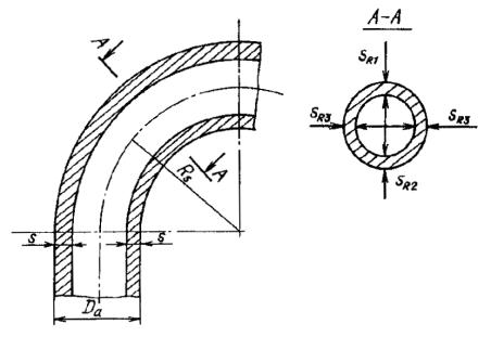
Fig. 4.5.
Elbow
4.2.2.5. Toroidal
coefficients are calculated by formulas
K1 = (4Rs
+ Da)/(4Rs + 2Da); K2
= (4Rs - Da)/(4Rs –
2Da); K3 = 1.
4.2.2.6. For elbows,
the design wall temperature which does not exceed 623 K (350 °C) for carbon and
silicon-manganese steels, 673 K (400 °C) for chromium-molybdenum-vanadium
steels, 723 K (450 °C) for corrosion-resistant steels of austenitic class, the
shape coefficients are determined by the formulas
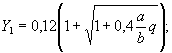
Y2 = Y1;
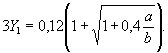
For elbows of
the same steel, but at a wall temperature of at least 673 K (400 °C), 723 K
(450 °C) and 798 K (525 °C), respectively, the shape coefficient is determined
by the formulas
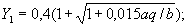
Y2 = Y1;
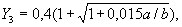
where a is
out-of-roundness of the cross section of the elbow, determined according to the
Codes,%; 

For elbows,
the design temperature of which is between the above values, the coefficients Y1,
Y2, Y3 are determined by linear
interpolation depending on the temperature value. In this case, the coefficient
values corresponding to the specified boundary temperatures are assumed as
reference.
If the
obtained values of coefficients Y1, Y2, Y3
are less than one, they should be assumed to be equal to one.
If b
< 0.03, values of the coefficients Y1, Y2,
Y3 are assumed to be equal to the value obtained when b
= 0.03. If the calculated value is q > 1, then it is assumed that q
= 1.
4.2.2.7. It is
allowed to round value of sR + c down to a value not
exceeding 3% of the nominal wall thickness.
4.2.2.8. At the ends
of pipes being bored for butt welding, the wall may be thinned by 10% of the
design thickness, provided that the total length of the bored section will not
exceed the smaller of the values of 5sR or 0.5Da.
4.2.2.9. Permissible
pressure for a cylindrical header, nozzle, pipe, and elbow is determined by the
formulas:
during design
after manufacture
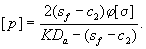
Coefficient K
is assumed to be: for cylindrical header, nozzle and pipe K = 1; for
elbow K = max{K1Y1; K2Y2;
K3Y3}.
4.2.3. Round flat
heads and lids.
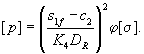
4.2.3.1. The design
thickness of the round flat heads and lids (Table 4.3), operating under
internal and external pressures, is determined by the formula
This formula
is applicable provided that
(s1
- c)/DR ≤ 0.2.
4.2.3.2. The nominal
thickness of round flat heads and lids operating under internal and external
pressures shall satisfy the condition
s1 ≥ s1R
+ c.
4.2.3.3. In all
cases of attaching a flat round head to the shell, the head thickness shall be
equal to or greater than the thickness of the shell, calculated according to
the formula in item 4.2.1.2.
Table 4.3. Values
of design diameter DR and coefficient K0
depending on the connection
|
Type
|
Connection
|
Design
diameter
|
K0
|
|
1
|
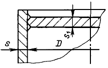
|
DR = D
|
0.53
|
|
2
|
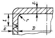
|
DR = D
- r
|
0.44

|
|
0.47

|
|
3
|
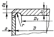
|
DR = D
|
0.47
|
|
4
|
|
DR = D4
|
0.6
|
|
5
|
|
DR = D2
|
0.45
|
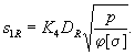
4.2.3.4.
Values of coefficient K4 in the formula in item 4.2.3.1
are determined depending on the design of heads and lids according to the
formula
K4 = K0x,
where coefficient K0
is assumed in accordance with Table 4.3.
The
coefficient of x, taking into account the rigidity of the connection of
a flat head with a cylindrical shell, is determined by the formula
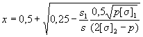
(if when calculating the
value of x < 0.76, then it is assumed that x = 0.76), where
[σ]1, [σ]2 are nominal permissible stresses for the
materials of the head and cylindrical shell, respectively.
For lids it is
assumed that x = 1.0.
Bending radius
r specified in Table 4.3 is assumed in accordance with the design
documentation.
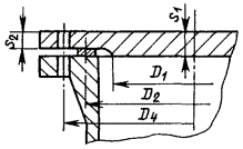
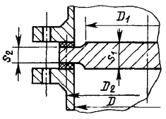
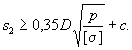
4.2.3.5. Thickness s2
for types of joints 3 and 5 (Table 4.3) shall satisfy the condition
For joint type
4 (Table 4.3)
s2 ≥ 0.75s1.
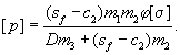
4.2.3.6. Permissible
pressure during design and after manufacture of round heads and lids operating
under internal and external pressures is determined by the formulas:
during design
after manufacture
4.3. STRENGTH REDUCTION
COEFFICIENTS AND STRENGTHENING OF HOLES
4.3.1. Strength
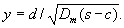
reduction by a single hole.
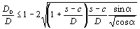
4.3.1.1. A single
hole is a hole the edge of which is distant from the edge of the nearest hole
along the middle surface for a distance more than 
If the outer
diameter is nominal, then the mean diameter is
Dm = 2Bk
+ s,
where Bk
is the distance from the point of intersection of longitudinal axis of the hole
or nozzle with the shell axis to the conditional point of intersection of
longitudinal axis of the hole with the inner forming part (see e.g. Fig. 4.2).
If the internal diameter is nominal, then
Dm = D +
s.
4.3.1.2. A
non-strengthened hole is a hole that has no strengthening in the form of a
nozzle with a wall thickness exceeding that required by calculation for the
design pressure; welded cover plate; local thickening of the shell around the
hole or flanged collar (upset neck), as well as a hole in which pipes are beaded.
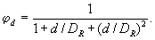
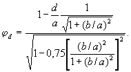
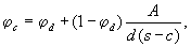
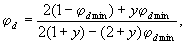
4.3.1.3. The
reduction coefficient of strength of a cylindrical, conical and spherical
shell, or a convex head weakened by non-strengthened single hole, is determined
by the formula

If the
calculated value of φd is > 1, then it is assumed that φd
= 1.
For flat heads
and lids
Diameter of
holes d in the calculations is assumed as:
1) for round
holes for beading pipes, for welding nozzles to the shell surface and for holes
closed by a lid, – equal to the diameter of holes in shells:
2) for
non-circular holes with an aspect ratio along symmetry axes of not more than
2:1 – equal to the largest clear size in the longitudinal direction for holes
in cylindrical and conical shells, and equal to the largest clear size in each
direction for spherical shells and convex heads;
3) for round
holes with a penetrating nozzle connected to the shell by a weld with full weld
penetration of the shell wall – equal to the internal diameter of the nozzle;
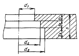
Fig. 4.6.
Diagram for determining the nominal hole diameter for a stepped hole
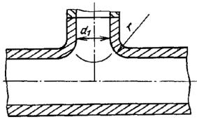
Fig. 4.7.
Diagram for determining the nominal hole diameter in a T-joint with a flanged
collar
4) for holes
with different diameters on the wall thickness – equal to the nominal diameter
determined by the formula
d = (d1s1
+ d2s2 + d3s3)/s,
where d1,
d2, d3, s1, s2,
s3, s are shown in Fig. 4.6;
5) for
T-joints with a flanged collar (upset neck) – equal to the nominal diameter
determined by the formula
d = d1
+ 0.5r,
where d1,
r are dimensions shown in Fig. 4.7.
Value of
diameter DR is assumed depending on the design of heads and
lids in accordance with Table 4.3.
4.3.1.4. The largest
permissible diameter of a non-strengthened single hole in shells is determined
by the formula
where 
Values of
coefficients m1, m2, m3
for shells and heads are given in Table 4.2.
4.3.1.5. If hole
diameter d exceeds permissible diameter d0 defined by
the formula in item 4.3.1.4, then this hole shall be strengthened with
the help of thickened nozzles, welded cover plates, local thickening of shell
around the hole, or by combining the said methods. At the same time, the
cross-sectional area of the strengthening components is equal to the sum of the
cross-sectional areas of nozzles and cover plates used for strengthening, as
well as of deposited metal for welding, i.e.
ΣА = Ac
+ An + Aw,
where Ac,
An, Aw are the cross-sectional areas of the
strengthening nozzle, welded cover plate and welded joints, respectively.
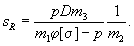
4.3.1.6. The
cross-sectional area of strengthening components shall satisfy the condition
ΣA ≥ (d
- d0)s0.
If, however,
the use of the above methods is not enough to strengthen the hole, or their use
is irrational for constructive reasons, the shell wall thickness shall be
increased, which will lead to corresponding changes in φ0 and d0
and to reduction of area ΣA required for strengthening.
Thickening of
shell around the hole (welding the saddle into the cylindrical shell) shall be
considered when determining the strengthening area as a cover plate.
4.3.1.7. The
reduction coefficient of wall strength of a cylindrical, conical and spherical
shell or a convex head, weakened by single strengthened hole, determined by the
formula
where φd
is the coefficient defined by the formula in item 4.3.1.3.
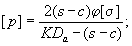
4.3.1.8. If it is
necessary to strengthen a single hole to achieve a predetermined value of the
strength reduction coefficient φ, the area of strengthening components of the
cross section can be determined without calculating the permissible diameter of
the hole according to the condition
where φd
is the coefficient defined by the formula in item 4.3.1.3.
4.3.1.9. If the
strengthening component is made of a material with a smaller value [σ] than
that of the shell material, then the calculated area of this strengthening
component shall be multiplied by the ratio of the nominal permissible stresses
for the shell materials and strengthening component.
A higher value
of [σ] for the material of strengthening component compared to [σ] for the
shell material is not taken into account in the calculation.
4.3.1.10. The
cross-sectional area of a strengthening nozzle (Fig. 4.8) is determined
by:
Fig. 4.8.
Diagram of strengthening cross-sections
Fig. 4.9.
Diagram of welded cover plate seams
for the area located
outside the shell (head),
Ac = 2hc(sc
- s0c - cc);
for the area located
inside the shell (head),
Ac = 2hc(sc
- cc).
In the latter
case, the increase in corrosion is taken into account on the outer and inner
surfaces of the nozzle.
Diagram of
strengthening cross-sections and welds of a welded cover plate are shown in
Fig. 4.8 and 4.9.
4.3.1.11. The
height of strengthening area of the nozzle is assumed according to Fig. 4.8,
but not more than
4.3.1.12. Nominal
thicknesses of the walls of shell and nozzle s and sc
are determined respectively by items 4.2.1 and 4.2.2. Minimum
design wall thickness of shell and nozzle s0 and s0c
are determined by the same formulas when φd = 1 and c
= 0.
Nominal wall
thickness of the nozzle shall not exceed the nominal wall thickness of the
shell.
4.3.1.13. The
cross-sectional area of strengthening welded cover plate is determined by the
formula
An = 2bnsn.
Width of cover
plate bn is assumed according to Fig. 4.9, but not
more than

Thickness of
cover plate sn is recommended to be assumed as no more s.
If sn > s, it is recommended to install the cover
plate outside sn1 and inside sn2
the vessel. Along with this sn1 + sn2
> 2s is not allowed.
4.3.1.14. Dimensions
of welds of the cover plate shall meet the condition
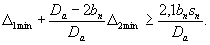
Dimensions of
welds of the nozzles shall meet the conditions
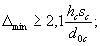 ∆min
≥ sc.
∆min
≥ sc.
The area of
strengthening cross-section of a single weld is determined by the formula
Aw = l1l2.
4.3.1.15. The
calculation methods given in item 4.3.1 are applicable for determining
the sizes of the strengthening components of cylindrical and conical shells,
convex and flat heads with round and oval holes.
The limits of
applicability of the calculation formulas are limited by the ratios of sizes
given in Table 4.4.
In Table 4.4,
DK is the internal diameter of a conical shell in
cross-section penetrating the hole.
Design hole
diameter dR is determined by the formulas:
for a round hole or
nozzle in the cross-section of shell
dR = d;
for conical shells in
the longitudinal section of shell
dR = d/cos2
α;
for hillside nozzles of
cylindrical shells and for all nozzles in hemispherical heads
dR = d/cos2
γ,
where γ is the angle
between the axis of a nozzle and the normal line to the surface of shell or
head;
Table 4.4. Limits
of applicability of calculation formulas
|
Parameters
|
In
cylindrical shells
|
In conical
shells (adapters and heads)
|
In
elliptical and hemispherical heads
|
|
Diameter ratio
|

|

|

|
|
Ratio of shell or head
wall thickness to diameter
|

|

|

|
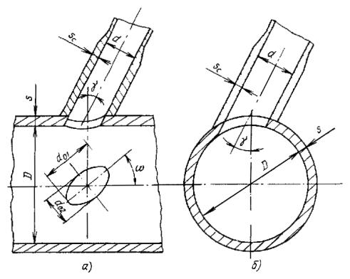
Fig. 4.10.
Hillside nozzle:
a – in the
longitudinal section of a shell; b – in the cross-section of a shell
for a hillside nozzle
hole when the major axis of the oval hole makes angle ω with the surface
generator of the shell (Fig. 4.10),
dR = d/(1
+ tg2 γ cos2 ω);
for a displaced nozzle
hole on the elliptical head (Fig. 4.11)
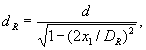
where the design
internal diameter of the elliptical head is determined by the formula
4.3.1.16. The given
method of determining the area of strengthening sections is applicable under
the conditions:
1) angle γ
between the axis of a nozzle and the normal line to the shell surface is within
15° (Fig. 4.10);
2) for
displaced nozzles on elliptical and hemispherical heads, the angle γ shall not
exceed 45° (Fig. 4.11);
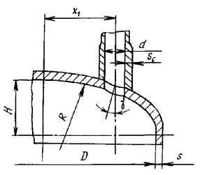
Fig. 4.11.
Displaced nozzle on elliptical head
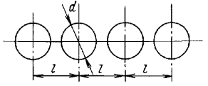
Fig. 4.12.
Longitudinal row of holes with the same pitch
3) the
distance from the head edge to the nozzle axis measured by the projection shall
be at least 0.1D + d/2.
4.3.2. Decrease in
strength with attenuation of a row of holes.
4.3.2.1. The
diameters and pitches of holes used in the formulas of this Section are
determined from the median surfaces of barrel sheets.
4.3.2.2. The row of
holes shall mean the holes, the distance between the edges of which does not
exceed the values 
4.3.2.3. The
coefficient of strength reduction in the longitudinal row of holes with the
same pitch (Fig. 4.12) in cylindrical and conical shells, or in the
number of any direction in elliptical and spherical shells is determined by the
formula
φd
= (l – d)/l.
4.3.2.4. The
coefficient of strength reduction with a circumferential (transverse) row of
holes with the same pitch (Fig. 4.13) in cylindrical and conical shells
is determined by the formula
φd
= (l1 – d)/l1.
4.3.2.5. When
staggered arrangement of holes (Fig. 4.14)
in cylindrical and
conical shells, determine three/values of the coefficient of strength reduction
by the formulas:
in longitudinal
direction
φd
= (2a – d)/(2a);
in circumferential
(transverse) direction
φd
= (2b – d)/b;
Fig. 4.13.
Transverse row of holes with the same pitch
cantwise
The smaller of
the values obtained are assumed as a design strength reduction coefficient
according to the formulas of this item.
4.3.2.6. For the
in-line arrangement of holes (Fig. 4.15), the value of the strength
reduction coefficient is assumed as the smallest of the values obtained for
longitudinal and transverse rows of holes.
4.3.2.7. When
unequal pitches between the holes (Fig. 4.16) or (and) unequal diameters
of the holes, the strength reduction coefficient φd is
assumed to be the smallest value of the strength reduction coefficients for
each pair of adjacent holes. Diameter of the hole is assumed to be equal to the
arithmetic mean value of diameters of adjacent holes in a row.
4.3.2.8. For flat
heads and lids with multiple holes, the minimum value of the strength reduction
coefficient shall be determined by the formula
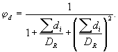
The maximum
sum of chord lengths of holes Σdi in the most weakened
diametrical section of a flat head or lid is determined in accordance with Fig.
4.17 according to the formula
Σdi
= max{(d1 + d3); (b2 + b3)}.
4.3.2.9. If several
single holes are located in the same direction with a row of holes, the
smallest value of strength reduction coefficient is assumed from the values for
a single hole and for a row of holes.
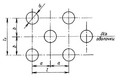
Fig. 4.14.
Staggered arrangement of holes
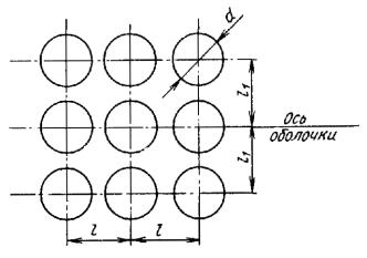
Fig. 4.15.
In-line arrangement of holes
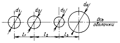
Fig. 4.16. Row
of holes with unequal holes and pitches
4.3.2.10. If the axis
of a row of holes does not intersect the center of a single hole, and the angle
between the axis of a row and a straight line connecting the center of this
hole to the center of the next one does not exceed 15°; then when determining
the strength reduction coefficient, this hole is attributed to the row.
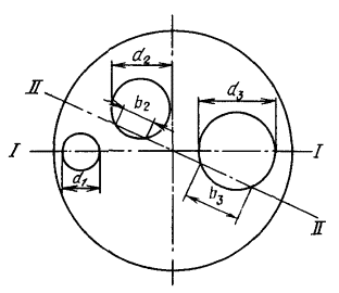
Fig. 4.17.
Head or lid with unequal holes and pitches
4.3.2.11. If the
axis of a row passes through a non-circular hole, the diameter of this hole is
assumed to be the largest size, determined by the axis of a row or a straight
line passing through the center of the non-circular hole with a deviation from
the row by an angle of up to 15°.
4.3.2.12. If each of
the holes forming a row has different strengthening components, the strength
reduction coefficient of such a row is determined as the minimum value for each
pair of adjacent holes by the formula
where φd
is determined by the formulas of items 4.3.2.3 - 4.3.2.5.
4.3.2.13. If it is
necessary to strengthen the holes in a row to a predetermined value of the
strength reduction coefficient φ, the cross-sectional area of the strengthening
components is determined according to the condition
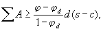
where φd
is determined by the formulas of items 4.3.2.3 - 4.3.2.5.
4.3.2.14. The
cross-sectional area of strengthening nozzles for the shell, weakened by a row
of holes with various-sized nozzles, is assumed as follows:
for the area located
outside the shell (head),
Ac = hc1(sc1
– s0c1 – cc1) + hc2(sc2
– s0c2 – cc2);
for the area located
inside the shell (head),
Ac = hc1(sc1
– cc1) + hc2(sc2
– cc2),
where indices 1 and 2
refer to two adjacent holes.
4.3.2.15. If the row
consists of only two holes, the strength coefficient is determined by the
formula
where φdmin
is the strength reduction coefficient for a row of holes, determined by the
formulas in items 4.3.2.2 - 4.3.2.5, 4.3.2.7.
The value of y
is determined by the formula
4.3.2.16. When an
arbitrary shape of strengthening components or nozzles, selected dimensions
shall satisfy the condition
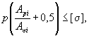
where Api
is the projection of an area under pressure p limited along the axis and
circumference of shell by value 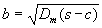 , and along the axis of
the nozzle by value hc assumed according to item 4.3.1.11
(Fig. 4.18); Aσi is the cross-sectional area of
the metal of the most loaded part limited by values b and hc
(Fig. 4.18).
, and along the axis of
the nozzle by value hc assumed according to item 4.3.1.11
(Fig. 4.18); Aσi is the cross-sectional area of
the metal of the most loaded part limited by values b and hc
(Fig. 4.18).
4.3.3. Strength
reduction coefficient of welded joints.
4.3.3.1. Strength
reduction coefficient of butt, corner, and T-shaped welded joints φw
is selected depending on the amount of flaw-detective control in accordance
with Table 4.5.
For products
from chromium-molybdenum-vanadium and high-chromium steels up to a temperature
of 783 K (510 °C), φw is assumed according to Table 4.5,
and at a temperature of 803 K (530 °C) or more φw = 0.7
irrespective of the scope of control. At design temperatures 783 K (510 °C) to
803 K (530 °C), the value of φw is determined by linear
interpolation.
Table 4.5. Values
of strength reduction coefficients of welded joints
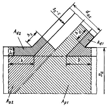
Fig. 4.18.
Diagram of design areas of strengthening components
If the welded
joint of pipes made of chrome-molybdenum-vanadium rolled, forged and drilled,
or centrifugally cast steels with a machined inner surface is loaded with
bending loads and operates at temperatures up to 783 K (510 °C), then
irrespective of the scope of control, for rolled pipes φw1
shall be assumed as 0.9 and for machined centrifugally cast pipes φw2
= 1. At a temperature of 803 K (530 °C) or more, φw1
= 0.6 and φw2 = 0.7, respectively. Within the
range of temperatures from 783 K (510 °C) to 803 K (530 °C), linear
interpolation is allowed to determine φw1 or φw2.
4.3.3.2. The
strength reduction coefficient of annular welded joints of cylindrical and
conical shells loaded with pressure is assumed to be equal to one.
4.3.3.3. If the
distance from the edge of any hole to the axis of a weld in the direction
perpendicular to the design direction is as follows,
the design strength
reduction coefficient is determined as a product of the strength reduction
coefficient of a welded joint and the strength reduction coefficient of a hole
φ = φdφw
or φ = φcφw.
In case the
distance between the axis of the weld and the edge of the nearest hole is
the design strength
reduction coefficient is assumed as the minimum value of φd,
φc or φw. For seamless parts φ = φd
or φ = φw. For welded parts without holes φ = φw.
4.4. FLANGES, PRESSURE
RINGS, AND FASTENERS
The
recommended method for calculation for selection of basic dimensions of
flanges, pressure rings, and fasteners is given in Appendix 10.
5. CHECKING CALCULATION
5.1. GENERAL
5.1.1. Checking
calculation is carried out after performing the calculation for selection of
basic dimensions of the calculated components according to their nominal
dimensions.
5.1.2. Checking
calculation is carried out with due regard to all design loads and all design
modes of operation. A group of modes can be included in one design mode if
external loads and temperatures of these modes do not differ by more than 5%
from the accepted design values.
5.1.3. The main design loads are:
internal or external
pressure;
weight of a product and
its content
additional loads (weight
of attached products, pipeline insulation, etc.);
forces from the reaction
of supports and pipelines;
thermal impacts;
vibration loads;
seismic loads.
5.1.4. The main design modes of operation are:
tightening of bolts and
pins;
start-up;
steady-state mode;
operation of the
emergency protection system;
reactor power change;
shutdown;
hydraulic or pneumatic
test;
abnormal operation;
emergency.
5.1.5. The
checking calculation uses physical and mechanical properties of the base metal
and welds specified in the state or industry standards or specifications. In
the absence of the necessary data in these documents, it is allowed to use the
data given in Tables P1.1 - P1.4 of Appendix 1 and
Appendix 6.
5.1.6. The
regulations do not regulate the methods used to determine design loads,
internal forces, displacements, stresses and deformations of the calculated
components. The selected method shall take into account all design loads for
all design cases and provide an opportunity to determine all necessary
calculation groups of stress categories.
Responsibility
for the selection of a method lies with the organization which performed the
appropriate calculation or experiment. Recommended methods for calculating some
typical assemblies and parts are given in Appendix 5.
5.1.7. During the
checking calculation, all stresses in the structure are divided into
categories. Stresses belonging to different categories are grouped into groups
of stress categories, which are compared with permissible stresses.
5.1.8. During the
checking calculation of the deposited or clad walls, the stresses in the wall
and deposit welding are considered with due regard to temperature stresses
caused by the difference in the coefficients of linear expansion of the base
metal and deposit welding.
5.2. CLASSIFICATION OF
STRESSES
5.2.1. The
following main categories of stresses are used for checking calculation:
σm –
general membrane stresses;
σmL –
local membrane stresses;
σb –
general bending stresses;
σbL –
local bending stresses;
σT –
general temperature stresses;
σTL –
local temperature stresses;
σc –
compensation stresses ;
σ mw –
mean tension stresses over bolt or pin section caused by mechanical loads.
Additional
stress categories used in performing calculations included in the checking
calculation are specified directly in the relevant subsections.
For
convenience of the calculations, below there are examples of the separation of
stresses by categories.
5.2.2. An example
of stresses belonging to the category of general membrane stresses is the mean
tension (or compression) stresses across the wall thickness of a cylindrical or
spherical shell, caused by the action of internal or external pressure.
5.2.3. Examples of
stresses classified as local membrane stresses are:
1) membrane
stresses from mechanical loads in the areas of connection of shells and
flanges;
2) membrane
stresses from mechanical loads in the areas of connection of branch pipes and
supports to vessels.
5.2.4. Examples of
stresses classified as general bending stresses are:
1) bending
stresses caused by external forces and moments acting on the vessel or pipeline
as a whole;
2) bending
stresses caused by pressure acting on flat lids;
3) bending
stresses in pressure rings and flanges of detachable joints caused by
tightening of bolts and pins.
5.2.5. Examples of
stresses classified as local bending stresses are:
1) bending
stresses caused by pressure in the areas of connection of various components
(flange and cylindrical shell of body, connection of body shell and head,
etc.);
2) bending
stresses in pipelines in the area of flange connection caused by tightening of
bolts and pins.
5.2.6. Examples of
stresses classified as general temperature stresses are:
1) stresses
caused by axial temperature differences in cylindrical shell;
2) linear part
of stresses in components in the connection areas (flange and cylindrical part
of vessel; branch pipe and vessel body; pipeline and flange; tube plate and
attached tubes, etc.);
3) stresses
caused by temperature differences across the thickness of flat heads and lids;
4) stresses in
butt joints of cylindrical shells made of dissimilar materials.
5.2.7. Examples of
stresses classified as local temperature stresses are:
1) stresses in
the central part of long cylindrical or spherical shells caused by temperature
differences across the wall thickness, with the exemption of the linear
component of stresses specified in 2) of item 5.2.6;
2) stresses in
small areas of overheating (or cooling) in the wall of a vessel or pipeline;
3) stresses in
anti-corrosion coating and other bimetallic components caused by the difference
in coefficients of linear expansion of materials.
5.2.8. Examples of
stresses classified as compensation stresses are:
1) tension (or
compression) stresses caused by constraining free expansion of a pipeline;
2) torsional
and bending stresses in pipelines caused by homing action of a pipe.
5.2.9. Examples of
stresses classified as local stresses in concentration areas are stresses in
the areas of holes, fillets, threads, etc. caused by thermal and mechanical
forces, determined with due regard to the stress concentration coefficient.
5.2.10. Checking
calculation determines the stresses of each calculation group of the stress
category, according to which the reduced stresses are determined, compared with
the corresponding permissible stresses.
5.2.11. Based on
the analysis of the existing loads and temperature fields, the most stressed
areas of vessels and pipelines shall be selected, and for different design
cases these areas may be different.
5.2.12. Groups of
categories of stresses and their designations in relation to various types of
structures used in the calculations for static and cyclic strength are given in
Table 5.1, and for calculated zones – in Table 5.2.
5.2.13. The most
typical examples of groups of categories of stress in structures are given in
Table 5.1.
5.3. STRESS CALCULATION
PROCEDURE
5.3.1. Based on
the analysis of operating conditions of components of structure, a typical
physically possible sequence of operating operation and loading modes is
established, including test conditions and abnormal operation. Operation and
loading modes carried out between start-up and outage, for example, operation
of emergency protection, shall be located between the specified modes.
5.3.2. For the
most loaded areas of the components of structure, the elastic calculation
determines the values of six components of stresses without taking into account
concentration for the adopted coordinate system (Cartesian, cylindrical or
spherical) and the adopted sequence of operation and loading modes in time.
The values of
main stresses are determined according to the six components of stress state.
The largest main stress is assigned an index i, and two others – indices
j, k (σi > σj > σk),
thus fixing the main sites.
5.3.3. On the
selected fixed main sites for the entire adopted sequence of operation and
loading modes in time, the dependences of the change in main stresses are
determined σi, σj, σk.
5.3.4. The values
of reduced stresses (σ) are determined for the moments of time t1,
t2, ..., tl, ..., tm,
where the increase (decrease) in the absolute value of any component of the
main stresses is replaced by their decrease (increase) according to the
formulas
 (5.1)
(5.1)
Table 5.1. Examples
of groups of construction stress categories
|
Construction
type
|
Design
group of stress categories
|
Designation
of calculation group of stress categories
|
Designations
of components of stress categories included in this calculation group
|
|
Bodies of reactors,
steam generators and vessels
|
Reduced general
membrane stresses
|
(σ)1
|
σm
|
|
Reduced stresses
determined by the sums of the components of general or local membrane and
general bending stresses
|
(σ)2
|
[σm
or σmL] + σb
|
|
Range of reduced
stresses determined by sums of components of general or local membrane
stresses, general and local bending and general temperature and compensation
stresses
|
(σ)RV
|
[σm
or σmL] + σb + σbL + σT
+ [σcm or σcmL] + σcb +
τcs
|
|
Amplitude of reduced
stresses determined by the sums of the components of general or local
membrane stresses, general and local bending stresses, general and local
temperature and compensation stresses with due regard to stress concentration
|
(σaF)V
|
[σm
or σmL] + σb + σbL + σT
+ σTL [σcm or σcmL] + σcb
+ τcs with due regard to stress concentration
|
|
Pipelines
|
Reduced general membrane
stresses
|
(σ)1
|
σm
|
|
Reduced stresses
determined by the sums of the components of general or local membrane and
general bending stresses
|
(σ)2
|
[σm
or σmL] + σb
|
|
Range of the reduced
stresses determined by the sums of the components of general or local
membrane stresses, general and local bending stress, general temperature
related stresses, and compensation stresses of membrane, torsion and bending
|
(σ)RK
|
[σm
or σmL] + σb + σbL + σT
+ [σcm or σcmL] + τcs +
σcb
|
|
Amplitude of reduced
stresses determined by the sums of the components of general or local
membrane stresses, general and local bending stresses, general and local
temperature stresses, compensation stresses of membrane, torsion and bending
with due regard to stress concentration
|
(σaF)K
|
[σm
or σmL] + σb + σbL + σT
+ σTL [σcm or σcmL] + τcs
+ σcb with due regard to stress concentration
|
|
Compensating devices
(toroidal, bellows, etc.)
|
Reduced general
membrane stresses
|
(σ)1
|
σm
|
|
Amplitude of reduced
stresses determined by the sums of the components of general or local
membrane stresses, general and local bending stresses, general and local
temperature stresses with due regard to stress concentration
|
(σaF)V
|
[σm
or σmL] + σb + σbL + σT
+ σTL with due regard to stress concentration
|
|
Bolts and pins
|
Mean tension stresses
over bolt or pin section caused by mechanical loads
|
(σ)1
|
σmw
|
|
Mean tension stresses
over bolt or pin section caused by mechanical loads and temperature impacts
|
(σ)3w
|
σmw
+ σT
|
|
Reduced stresses
determined by sums of components of mean tension stresses over bolt or pin
section and general bending stresses caused by mechanical loads and
temperature impacts, as well as torsional stresses
|
(σ)4w
|
σmw
+ σT + σbw + τsw
|
|
Amplitude of reduced
stresses determined by sums of components of mean tension stresses over bolt
or pin section and general bending stresses caused by mechanical loads and
temperature impacts, torsional stresses and general and local temperature
stresses taking into account stress concentration in thread
|
(σaF)w
|
σmw
+ σbw + σT + σTL + τsw
with due regard to stress concentration
|
Table 5.2. Examples
of groups of categories in calculated areas of structures
|
Calculated
area
|
Type of
loading
|
Category
of determined stresses
|
Design
group of stress categories
|
|
Cylindrical portion
(smooth portion)
|
Internal pressure
|
General membrane
|
(σ)1
|
|
Internal pressure,
temperature difference along the length
|
General membrane +
general temperature
|
(σ)RV
|
|
Internal pressure,
temperature difference along the length, temperature difference through the
wall thickness
|
General membrane +
general temperature + local temperature
|
(σaF)V
|
|
Area of flange
connection with vessel cylindrical portion
|
Internal pressure
|
Local membrane
|
(σ)2
|
|
Internal pressure,
temperature field in flange, temperature field in vessel cylindrical portion
|
Local membrane + local
bending + general temperature
|
(σ)RV
|
|
Local membrane + local
bending + general temperature + local stresses in concentration areas
|
(σaF)V
|
|
Flat lid of vessel
with holes
|
Internal pressure
|
General bending
|
(σ)2
|
|
Internal pressure,
temperature field
|
General bending +
general temperature
|
(σ)RV
|
|
General bending +
general temperature + local temperature + local stresses in concentration
areas
|
(σaF)V
|
|
Area of connection of
flanges with elliptical or torospheric lids or heads
|
Internal pressure
|
Local membrane
|
(σ)2
|
|
Internal pressure,
temperature field in the flange, temperature field in the lid (head),
tightening of pins
|
Local membrane + local
bending + general temperature
|
(σ)RV
|
|
Local membrane + local
bending + general temperature + local temperature + local stresses in
concentration areas
|
(σaF)V
|
|
Elliptical or
torospheric lids or heads with holes
|
Internal pressure
|
General membrane
|
(σ)1
|
|
General membrane +
general bending
|
(σ)2
|
|
Internal pressure,
temperature field
|
General membrane +
general bending + general temperature
|
(σ)RV
|
|
General membrane +
general bending + general temperature + local temperature + local stresses in
concentration areas
|
(σaF)V
|
|
Area of connection of
vessel cylindrical portion with head
|
Internal pressure
|
Local membrane
|
(σ)2
|
|
Internal pressure,
temperature fields in vessel cylindrical portion and head
|
Local membrane + local
bending + general temperature
|
(σ)RV
|
|
Local membrane + local
bending + general temperature + local temperature + local stresses in
concentration areas
|
(σaF)V
|
|
Welding area of branch
pipes, nozzles or pipes to the vessel (in the body)
|
Internal pressure
|
Local membrane
|
(σ)2
|
|
Internal pressure,
temperature fields in the body and in the welded component, the forces from
the pipeline (mechanical and from homing action)
|
Local membrane + local
bending + general temperature + compensation stresses
|
(σ)RV
|
|
Local membrane + local
bending + general temperature + compensation stresses + local temperature +
local stresses in concentration areas
|
(σaF)V
|
|
Branch pipe area
|
Internal pressure
|
General membrane
|
(σ)1
|
|
Internal pressure,
temperature fields in the body and in the welded component, the forces from
the pipeline (mechanical and from homing action)
|
General or local
membrane + general bending
|
(σ)2
|
|
General or local
membrane + general bending + local bending + general temperature +
compensation stresses
|
(σ)RV
|
|
General and local
membrane + general bending + local bending + general temperature +
compensation stresses + local temperature and local stresses in concentration
areas
|
(σaF)V
|
|
Pressure ring
|
Pin tightening,
internal pressure
|
General bending
|
(σ)2
|
|
Pin tightening,
internal pressure, temperature fields in pressure ring and vessel
|
General bending +
general temperature
|
(σ)RV
|
|
General bending +
general temperature + local temperature + local stresses in concentration
areas
|
(σaF)V
|
|
Pipelines
|
Internal pressure
|
General membrane
|
(σ)1
|
|
Internal pressure,
weight of pipeline
|
General or local
membrane + general bending
|
(σ)2
|
|
Internal pressure; weight
of pipeline, compensation forces
|
General or local
membrane + general bending + compensation stresses + local bending + general
temperature stresses
|
(σ)RK
|
|
General or local
membrane + general bending + compensation stresses + local bending + general
temperature stresses with due regard to local stresses in the concentration
area
|
(σaF)K
|
|
Tube boards
|
Internal pressure
|
General bending
|
(σ)2
|
|
Internal pressure,
temperature fields
|
General bending +
general temperature
|
(σ)RV
|
|
General bending +
general temperature + local temperature with due regard to local stresses in
the concentration areas
|
(σaF)V
|
|
Area of welding of
tube plates to vessel body
|
Internal pressure
|
Local membrane
|
(σ)2
|
|
Internal pressure,
temperature fields in the tube plate and vessel body
|
Local membrane + local
bending + general temperature
|
(σ)RV
|
|
Local membrane + local
bending + general temperature with due regard to local stresses in the
concentration areas
|
(σaF)V
|
|
Headers
|
Internal pressure
|
General or local
membrane
|
(σ)1
or (σ)2
|
|
Internal pressure,
temperature fields
|
General or local
membrane + general or local flexural + general temperature
|
(σ)RV
|
|
General or local
membrane + general or local bending + general temperature + local temperature
with due regard to local stresses in the concentration areas
|
(σaF)V
|
|
Area of connection of
nozzles or pipes with a header
|
Internal pressure
|
Local membrane
|
(σ)2
|
|
Internal pressure,
temperature fields in the body and welded component
|
Local membrane + local
bending + general temperature
|
(σ)RV
|
|
Local membrane + local
bending + general temperature + local temperature + local stresses in
concentration areas
|
(σaF)V
|
|
Annular seal
(compensator)
|
Internal pressure
|
General membrane
|
(σ)1
|
|
Internal pressure,
movement of lid or head and body, temperature fields in the compensator
|
General or local
membrane + general temperature + local bending + local stresses in the
concentration areas
|
(σaF)V
|
Under elastic
loading for initial t1 and final tm moments
of time σi = σj = σk = 0
or equal to a constant stress, such as weight stress.
5.3.5.
Determination of stresses by analytical methods, for example, according to the
theory of shells, is carried out in the sequence specified in items 5.3.1
- 5.3.4; determination of stresses by numerical methods in the elastic
area in the following order:
1) dependence
of local stresses is determined for the accepted sequence of operation modes
and loading;
2) nominal
stresses from mechanical and thermal loads are distinguished;
3) reduced
stresses are determined.
5.3.6. The (σ)RV
or (σ)RK stress range is determined by a checking calculation
for static strength according to the graphs of changes in reduced stress (σ)ij,
(σ)jk, (σ)ik for the whole process of
stress change, and is selected as the largest of the following values:
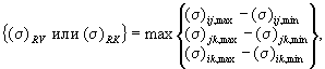 (5.2)
(5.2)
where (σ)ij,max,
(σ)jk,max, (σ)ik,max
are algebraically maximal, and (σ)ij,min, (σ)jk,min,
(σ)ik,min are algebraically minimal stresses for
the whole process of change of the corresponding reduced stresses.
In all cases
of elastic loading, the stress values
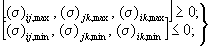 (5.3)
(5.3)
5.3.7. The general
process of change in time of reduced stresses (σ)ij, (σ)jk,
(σ)ik is a series of consecutive half cycles. Within each
half-cycle, the reduced stress varies monotonously. The moments of time
defining the ends of half cycles are denoted by 0, 1, 2, ..., l, ..., m.
The main
stresses σi, σj, σk, in
the general case distributed non-uniformly over the cross-sectional area (wall
thickness) of the component of structure As, are divided into
membrane σm and additional component, assumed as bending σb,
and are determined at specified moments using the formulas
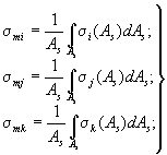 (5.4)
(5.4)
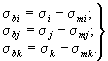 (5.5)
(5.5)
Reduced local
stresses (σL)ij, (σL)jk,
(σL)ik at the end of the lth
half-cycle are determined by the formulas
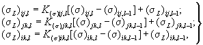 (5.6)
(5.6)
where K(σ)ij,l,
K(σ)jk,l, K(σ)ik,l
are concentration coefficients of reduced stresses for stresses (σ)ij,
(σ)jk, (σ)ik in a half-cycle from l
- 1 to l.
Coefficient K(σ)ij,l
is calculated, for example, by the formula
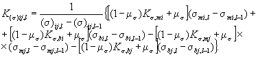 (5.7)
(5.7)
Here Kσ,mi,
Kσ,bi, Kσ,mj, Kσ,bj
are theoretical coefficients of concentration of membrane components σmi,
σmj and bending components σbi, σbj
are, respectively, determined experimentally, by handbooks, or with Appendix 3;
μσ is a coefficient depending on the constraint of deformation
corresponding to main stress σj in the direction of σi
and stress σi in the direction of σj. With
full constraint μσ = 0.3, and in its absence μσ = 0. If
the degree of constraint cannot be determined, then the calculation is
performed when μσ = 0 and μσ = 0.3. In this case, the
concentration coefficient is assumed as the largest of the two values obtained.

Fig. 5.1.
Graph of change of local reduced stress
To simplify
the calculation, it is allowed to assume Kσ,bi = Kσ,mi;
Kσ,bj = Kσ,mj and σmi
= σi; σmj = σj; σbi
= σbj = 0.
5.3.8. Change in
any local conditional elastic reduced stress (σF)l
is determined using the graph of change of corresponding reduced stress (σL)l.
An example of the graph is shown in Fig. 5.1.
If before a
moment in time l the stress (σL) was in the elastic
area (l = 2 in Fig. 5.1), then (σF)l
= (σL)l, and if at the moment of time l
the stress (σL)l is in the elastic plastic
area and at this moment acquires the highest absolute value among all the
preceding positive and negative stresses (σL), then (σF)l
is determined by the formula
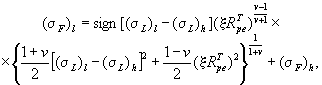 (5.8)
(5.8)
where in this case (σL)h
= (σF)h = 0, and x = 1.
In this case,
the moment in time is indicated by lb (lb =
4 and lb = 10), and work-hardening exponent v and
proportional limit RTpe are determined by the
formula
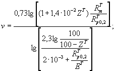 (5.9)
(5.9)
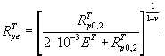 (5.10)
Work-hardening
exponent v is allowed to be selected as per Table 5.3 depending
on the value of RTp0.2/RTm
and ZT.
Table 5.3. Value
of work-hardening exponent v
|
RTp0.2/RTm
|
ZT, %
|
|
10
|
20
|
30 - 60
|
|
0.3
|
0.29
|
0.27
|
0.25
|
|
0.5
|
0.21
|
0.17
|
0.19
|
|
0.7
|
0.11
|
0.11
|
0.13
|
|
0.9
|
0.05
|
0.06
|
0.07
|
|
0.95
|
0.02
|
0.03
|
0.04
|
|
1.0
|
0.00
|
0.00
|
0.00
|
When
intermediate values of RTp0.2/RTm,
the values of v are determined by linear interpolation.
If a weld is
located in the are under consideration, then RTpe
and v values are assumed for the weld metal if they are smaller than for
the base metal.
At
temperatures above the Tt, the value of RTpe
is determined by the isochronous strain curve during the loading of the
component of structure during the considered half-cycle.
The duration
of a half-cycle is equal to the time of stress change from the minimum
(maximum) to the maximum (minimum) value. When calculating the stresses during
the start-up process, reach of standard conditions after any transient and
operation in the steady-state mode until the next transient at temperatures
above Mt, it is necessary to take into account the mean
operating time in the steady-state mode between the corresponding transients.
At
temperatures above Tt, the work-hardening exponent is
determined by the formula
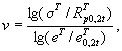
where RTp0.2t;
σT is a yield limit and stress corresponding to elastic
plastic deformation eT, assumed as per isochronic strain
curve for the duration and temperature of a half-cycle; eT0.2t
is deformation corresponding to the yield limit RTp0.2t;
eT is deformation corresponding to σT (at
least 2 %).
If before a
moment of time l the formula (5.8) was used at least once, then
to determine the stress (σF)l a half-cycle l,
h is considered, where lb ≤ h ≤ l.
When
increasing (decreasing) stress (σL) from a moment of time l
- 1 to l, index h is assigned to the lowest (highest) stress
value (σL). In this case, the stress values from (σL)h
to (σL)l-1 shall not exceed (or
be less than) the values of (σL)l.
If |(σL)l
- (σL)h| ≤ 2RTpe
(l = 7 in Fig. 5.1), then (σF)l
is determined by the formula
(σF)l
= (σL)l – (σL)h
+ (σF)h. (5.11)
If |(σL)l
- (σL)h| ≤ 2RTpe
(l = 5 and l = 8), then (σF)l
is determined by the formula (5.8), in which the coefficient x is
assumed to be equal to 2.
When the
temperature is variable during a half-cycle, the values of RTpe,
v are calculated for the maximum and minimum half-cycle temperatures
according to the corresponding values of RTp0.2,
RTm, ZT, ET.
The value of RTpe is assumed to be equal to the
half-sum of the corresponding values at the maximum and minimum half-cycle
temperatures, and the indicator v is taken to be equal to the minimum of
its values in the half-cycle temperature range. It is allowed to use values of RTpe,
v at the maximum half-cycle temperature.
Work-hardening
exponent v, when it is determined according to Table 5.3, is
assumed to be equal to its minimum value in the half-cycle temperature range.
It is allowed
to assume RTpe to be equal to RTp0.2,
and work-hardening exponent v = 0. In this case, the value of RTp0.2
is equal to the half-sum of the yield limits at the maximum and minimum
half-cycle temperatures, or to the yield limit at the maximum half-cycle
temperature.
Calculation by
the formula (5.8) is allowed to be applied under the following
conditions:
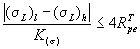 (5.12)
 (5.13)
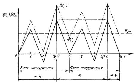
Fig. 5.2.
Graph of change of local conditional elastic reduced stress (σF)
for two identical adjacent stress units (σL):
* –
half-cycles between the highest values of (σL)lb;
** – other half-cycles
|
блок нагружения
|
loading unit
|
If when
calculating (σF)l and determining the graph
of its change, the formula (5.8) was used at least once, then two
identical stress change units shall be considered successively (σL)
(see an example in Fig. 5.2). In this case, the number of half-cycles
(cycles) of each type between absolutely highest values of (σL)lb
is assumed to be equal to the expected, when operating, number of load units
minus 1, the number of the rest is 1.
5.3.9. Local
conditional elastic reduced stress (σF) using an effective
concentration coefficient Kef is determined by the formula
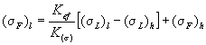 (5.14)
or
(σF)l
= Kef[(σ)l – (σ)h] + (σF)h.
(5.15)
5.3.10. Effective
local reduced stress concentration coefficient Kef is
determined by fatigue tests.
Geometry,
surface condition, nominal stresses and gradients of local stresses in the
concentration area of the tested component, model or sample; their material and
heat treatment; loading conditions (temperature, medium) shall correspond to
the full-size component of structure.
Stresses
without taking into account the concentration when determining Kef
shall not exceed the limits established for the corresponding categories of
stresses in the calculation of static strength.
Use of Kef,
when calculating local reduced stresses, shall be coordinated with the method
of processing experimental data in its determination.
When (σaL)
≤ RTp0.2, the effective stress
concentration coefficient is determined by the formula
Kef = 1 + q(Kσ
- 1), (5.16)
where q is the
coefficient of material sensitivity to stress concentration (q ≤ 1).
If (σaL)
= Kσ(σa) ≥ RT-1,
then coefficient q is calculated by the formula
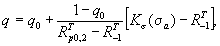 (5.17)
and if Kσ(σa)
< RT-1, then q is assumed to be equal to
q0, where q0 is the coefficient of material
sensitivity to stress concentration determined with the amplitude of local
stresses equal to the endurance limit RT-1 and
selectable according to Table. 5.4.
Table 5.4. Values
of coefficient of material sensitivity q0
|
RTp0.2/RTm
|
q0
|
Stress
concentration area in components of structures
|
|
0.4 - 0.8
|
1.0
|
Vessel support
devices, holes for pins for attaching lids to vessel bodies, holes of lids
and heads with a rounding radius of more than 40 mm
|
|
0.4
|
0.9
|
Tube plates,
curvatures, transition from pipelines to flanges with a rounding radius from
10 to 40 mm
|
|
0.6
|
0.95
|
|
0.8
|
1.0
|
|
0.4
|
0.7
|
Roundings at the tops
of slots and supporting clamps with a rounding radius from 4 to 10 mm
|
|
0.6
|
0.8
|
|
0.8
|
0.9
|
|
0.4
|
0.3
|
Metric thread of pins,
bolts, nuts with a rounding radius of less than 1 mm
|
|
0.6
|
0.6
|
|
0.8
|
0.8
|
Note. When
intermediate value of RTp0.2/RTm,
the value of q0 is determined by linear interpolation.
5.3.11. When
calculating reduced local conditional elastic stresses from mechanical and
thermal loads in welded joints with incomplete penetration performed with
austenitic electrodes and used to connect components of anti-corrosion jackets,
the effective axial stress concentration coefficient of any category shall be
determined depending on amplitude of bending σab and
uniformly distributed σam components of stresses without
taking into account concentration, by the formulas
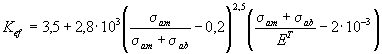
at 2 · 10-3 ≤
(σam + σab)/ЕM ≤ 4 · 10-3;
0.2 ≤ σam/(σam
+ σab) ≤ 1 and
Kef = 3.5 at (σam
+ σab)/ЕT ≤ 2 · 10-3; σam/(σab
+ σam) ≤ 0.2
or at σam
= 0 irrespective of σab.
For annular
membrane stresses, the concentration effect is ignored. Height of the weld
shall be no less than thickness of the thinnest of parts to be joined at the
weld. In case of occurrence of plastic cyclic deformations in
incomplete-penetration welded joints, the values of conditional elastic
stresses without taking into account concentration in the welded joint
cross-section shall be determined from elastic plastic calculation.
5.3.12. Local
conditional elastic stress (σF) in the thread of the threaded
connection is determined in accordance with item 5.3.8. Stresses (σL)
are calculated with due regard to the coefficient Kσ,
determined for metric thread, by the formula
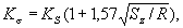 (5.18)
where KS
is a coefficient depending on the type of nut; Sz is a thread
pitch; R is a bending radius at the base of a coil.
For standard
compression nut, ratio KS = 1, and for tension-compression
nut with a length of the stretched zone equal to the diameter of threaded part,
KS = 0.75.
Coefficient KS
for intermediate lengths of stretched zone of the tension-compression nut is
set by linear interpolation.
When an
increase in the height of compression nut from 0.8 of the diameter of threaded
part to 1.25 and higher, the KS decreases from 1 to 0.9.
When
calculating the threaded part of a pin screwed into the body flange, the effect
on Kσ of the differences in mechanical properties of the
material of the pin and flange is taken into account. Moreover, with the length
of the screwed part of the pin equal to its diameter and more, coefficient KS
= 0.75.
In case of
differences in the stress limit of the materials of pin RTmw
and flange RTmf, the concentration coefficient is
determined by the formula
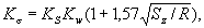 (5.19)
where the value of
coefficient Kw is determined according to Table 5.5.
Table 5.5 Value
of coefficient Kw
|
RTmf/RTmw
|
0.5
|
0.6
|
0.7
|
0.8
|
0.9
|
1.0
|
|
Kw
|
0.7
|
0.8
|
0.87
|
0.95
|
0.95
|
1.0
|
Local stress
(σF) in the thread may be determined using the effective
concentration coefficient Kef by the formula (5.14) or
(5.15). If stress (σL) does not go beyond the elastic
limits, then the coefficient Kef is determined by the formula
(5.16). If stress (σL) goes beyond the elastic limits,
then for a threaded connection with a metric thread made of steel with ZT
≥ 30 % with a controlled thread profile with a bending radius at the base of a
coil R, it is allowed to assume Kef = Kσ.
For controlled
metric threads with a hollow without bending made of steels with ZT
≥ 30 %, the value of Kef = 1.2Kσ, where Kσ
is a stress concentration coefficient in thread with pitch and bending radius R
= 0.11Sz.
5.3.13. When
calculating toroidal sealing compensators (TSC), the permissible number of
cycles for given local conditional elastic stresses is assumed as the minimum
of two values determined:
in the place of
compensator connection to massive parts (lid, body);
in the shell of
compensator between the connection points.
Local
meridional stress at the attachment point is determined (at 2Ro/s)
≥ 5, where Ro is a local outer curvature radius of the shell
cross section; s is a wall thickness) by multiplying the thermal and
mechanical force meridional stress on the outer surface calculated without
taking into account the concentration, as in a thin-walled shell, by the
effective concentration coefficient Kef.
For shells of
austenitic steels with a wall thickness s ≤ 6 mm, concentration
coefficient is determined by the formula Kef = 1.45 - 0.013R,
where R is a fillet radius at the attachment point, mm.
For non-smooth
fillet (ledge up to 2 mm at R ≥ 15 mm), the value of R is assumed
to be equal to zero. When determining hoop stresses, the concentration is not
taken into account.
In the area
between the connection points of a compensator if
2Ro/(s +
∆s1 + ∆s2) ≥ 3.5,
where ∆s1
and ∆s2 is the height of the butt weld reinforcement on
concave and convex TSC surfaces, respectively, the bending meridional stress is
determined by multiplying the bending meridional stress, calculated as in a
thin-walled shell, by the correction coefficients
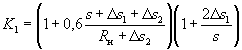
(concave surface) and
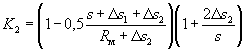
(convex surface), where Rl
- local inner curvature radius of the shell cross section.
5.3.14. When
determining local reduced stresses, it is allowed to present a typical timing
sequence of operation modes of operation and loading as separate blocks, with
due regard to the memory of the loading history during the transition from one
block to another.
5.3.15. The
stress cycles are formed so that each time the largest possible amplitude of
local reduced stress was obtained on three graphs of stress changes (σF)ij,
(σF)jk, (σF)ik
for the selected timing sequence of operating modes of operation and loading
from the remaining areas.
According to
the three graphs of local reduced stresses, the conditional elastic stress (σ*F)max,
largest in absolute value, is set for the whole process of stress changing.
5.4. CALCULATION
FOR STATIC STRENGTH
5.4.1. When
calculating the static strength, the fulfillment of the strength conditions for
the design loads specified in item 5.1.3, except for seismic and
vibration loads, and for all operating modes specified in item 5.1.4 is
checked.
5.4.2. Stresses
determined in calculation for static strength of equipment and pipeline
components shall not exceed values indicated in Table 5.6. Values of
[σ], [σ]c and [σ]w are determined in
accordance with the instructions in Section 3.
5.4.3. Mean
bearing stresses shall not exceed 1.57RTp0.2.
If the distance from the edge of the area of load application to the free edge
exceeds the size of the area on which the load acts, the permissible stresses
can be increased by 25%.
5.4.4. Mean
tangent stresses caused by mechanical loads shall not exceed 0.5[σ] (0.25RTp0.2
in threads).
5.4.5. Mean
tangent stresses caused by mechanical loads and temperature impacts shall not
exceed 0.65[σ] (0.32RTp0.2 in threads).
5.4.6. General
membrane tension during hydraulic (pneumatic) tests of pipelines must not
exceed 1.35[σ]Th, whereas the reduced stresses determined as
a sum of the components of general and local membrane stresses and general
bending stresses – 1.7[σ]Th. Stresses σmw
in bolts and pins shall not exceed 0.7RThp0.2.
5.4.7. When
assessing static strength over stress ranges (σ)RV or (σ)RK
(see Table 5.6), the maximum and minimum absolute values of the reduced stresses
included in the definition of this category shall not exceed RTm.
5.4.8. Meeting the
requirements of Table 5.6 and item 5.4.7 in terms of stress range
is not necessary in those cases when the distortion of the structure form,
which is possible during operation and which is associated with non-fulfillment
of the above requirements, can not affect the normal operation of the
calculated assembly (no violation of tightness of various joints, no jamming of
movable devices, no unacceptable distortion of the flow areas that determine
the coolant flow rate, no unacceptable deformations of mating parts,
etc.).
Necessity to
meet the requirements as per categories (σ)RV and (σ)RK
shall be established by the design (engineering) organization.
5.5.
CALCULATION FOR STABILITY
5.5.1. Cylindrical
shells under external pressure.
5.5.1.1. The
calculation is carried out for smooth cylindrical shells under the
comprehensive or lateral external pressure. When lateral pressure, there is no
pressure on the side surfaces of the shell.
5.5.1.2. Cylindrical
shells are considered to be smooth if their effective length has no
strengthened holes with a diameter exceeding d0 (see item 4.3.1.4),
ring and spiral stiffeners or other strengthening. Longitudinal or spiral
stiffeners with an angle of up to 30° to the generatrix are not considered as
strengthening from the external pressure effect.
5.5.1.3. A smooth
cylindrical shell at the effective length is considered.
If the
cylindrical shell at the sides is closed by welded convex heads, the length of
cylindrical shell, increased by the length of flanged cylindrical section and
by Hm/3 of each head, is assumed as the effective length.
Table 5.6.
Calculation group of stress categories
|
Construction
type
|
Design
case (mode)
|
(σ)1
|
(σ)2
|
(σ)3w
|
(σ)4w
|
(σ)RV
|
(σ)RK
|
|
Components of reactor
vessels, steam generators, tanks
|
NO
|
[σ]
|
1.3[σ]
|
-
|
-
|
(2.5 - RTp0.2/RTm)RTp0.2,
but no more than 2RTp0.2
|
-
|
|
AO
|
1.2[σ]
|
1.6[σ]
|
-
|
-
|
-
|
-
|
|
NPP
|
1.4[σ]
|
1.8[σ]
|
-
|
-
|
-
|
-
|
|
Pipelines
|
NO
|
[σ]
|
1.3[σ]
|
-
|
-
|
-
|
(2.5 - RTp0.2/RTm)RTp0.2,
but no more than 2RTp0.2
|
|
AO
|
1.2[σ]
|
1.6[σ]
|
-
|
-
|
-
|
|
Compensation devices
|
NO
|
[σ]
|
-
|
-
|
-
|
-
|
-
|
|
AO
|
1.2[σ]
|
-
|
-
|
-
|
-
|
-
|
|
Bolts and pins
|
NO
|
[σ]w
|
-
|
1.3[σ]w
|
1.7[σ]w
|
-
|
-
|
|
AO
|
1.2[σ]w
|
-
|
1.6[σ]w
|
2.0[σ]w
|
-
|
-
|
|
NPP*
|
1.4[σ]w
|
-
|
1.8[σ]w
|
2.4[σ]w
|
-
|
-
|
|
Guard tanka and
containments
|
Depressurization of
protected equipment or pipelines
|
[σ]c
|
1.3[σ]c
|
-
|
-
|
-
|
-
|
|
* Considered
only for reactor vessels.
|
For
cylindrical shell closed by flange joints or flat heads, the length of the
shell between flanges or between flat heads is assumed as the effective length.
5.5.1.4. Formulas
are applied under the following conditions:
0.005 ≤ (s - c)/Dm
≤ 0.1; Dm/L ≤ 3; a ≤ 2 %,
where a = 200(Damax
– Damin)/(Damax + Damin);
Damax, Damin are
maximum and minimum outer diameters measured in a single cross section of
cylindrical shell.
5.5.1.5. Critical
length
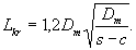
5.5.1.6. Critical
stress
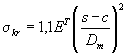 for L
≥ Lkr;
for L
≥ Lkr;
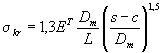 for Dm/3
< L < Lkr.
for Dm/3
< L < Lkr.
5.5.1.7. Critical
pressure
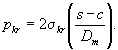
5.5.1.8. Permissible
external pressure
[pa]
= 0.5xpkr,
where correction
coefficient
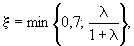 where
where 
5.5.1.9. Stability
of the cylindrical shell is ensured under the following condition
pa ≤ [pa].
5.5.2. The
cylindrical shell is under the axial force.
5.5.2.1. The
formulas are applicable for the calculation of smooth cylindrical shells
without longitudinal stiffeners.
Spiral
stiffeners at an angle of more than 60° to the generatrix are not considered as
strengthening from the axial force effect.
5.5.2.2. The
effective length of shell is assumed according to item 5.5.13.
5.5.2.3. Formulas
are applied under the following conditions:
0.05 ≤ (s – c)/Dm
≤ 0.2.
5.5.2.4. .Design
axial compression stress
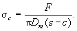
5.5.2.5. To
determine the value of the permissible stress, two values of the critical
stress are found:
stress of the first kind
– according to the condition of the general loss of stability of the
cylindrical component as a long rod;
stress of the second
kind – according to the condition of the local loss of stability of a
cylindrical thin-walled shell.
5.5.2.6. Critical
stress of the first kind
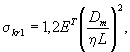
where η = 1 if both ends
of the cylindrical shell are hinged; η = 0.5 if both ends of the shell are
fully-fixed; η = 0.7 if one end of the shell is hinged, and the other is
fully-fixed.
5.5.2.7. Critical stress of the second
kind
σkr2
= 1.2ET(s - c)/Dm.
5.5.2.8. Permissible axial compression
stress
[σc]
= min{[σc]1; [σc]2},
where [σc]1
= 0.5x1σkr1; [σc]2
= 0.5x2σkr2,
correction coefficients
x1
= min{0.7; λ1/(1 + λ1)}, λ1 = RTp0.2/σkr1;
x2
= min{0.25; λ2/(1 + λ2)}, λ2 = RTp0.2/σkr2.
5.5.2.9. Stability
of the cylindrical shell is ensured under the following condition
σc
≤ [σc].
5.5.3. The
cylindrical shell under the joint action of external pressure and axial force.
5.5.3.1. The
formulas are applicable for smooth cylindrical shells without ring, spiral, or
longitudinal stiffeners and other types of strengthening (corrugations, etc.).
5.5.3.2. For the
case in question, the conditions given in items 5.5.1.1, 5.5.1.3,
5.5.1.4 shall be performed.
5.5.3.3. Stability
of the cylindrical shell is ensured under the following condition
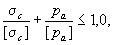
where the permissible external
pressure is determined according to item 5.5.1, and the design axial
compression stress σc and permissible axial compression
stress [σc] are determined according to item 5.5.2.
5.5.4. Convex
heads under external pressure.
5.5.4.1. The
formulas are designed to calculate the convex heads of hemispherical and
elliptical shapes, that are under pressure evenly distributed over the outer
surface.
The use of the
formulas for convex heads of spherical shape is allowed. In spherical
(dish-shaped) heads, the surface has the shape of a sphere segment.
5.5.4.2. Formulas
are applied under the following conditions:
0.005 ≤ (s - c)/Dm
≤ 0.1; Hm/Dm ≥ 0.2.
5.5.4.3. Critical
stress
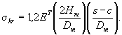
5.5.4.4. Critical
pressure
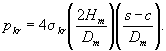
5.5.4.5. Permissible
external pressure
[pa]
= 0.5xpkr,
where correction
coefficient
x = min{0.15;
λ/(1 + λ)}, where λ = RTp0.2/σkr.
5.5.4.6. Stability
of the convex head is ensured if the condition of item 5.5.1.9 is
followed.
5.5.5. Conical
adapters under external pressure.
5.5.5.1. The
formulas are applicable for calculating the external pressure of smooth conical
adapters with angle of taper α satisfying the conditions of
0.005 ≤ (s – c)/D0m
≤ 0.1; 10 ≤ α ≤ 60°;
0.005 ≤ (s – c)/Dm
≤ 0.1,
where D0m
and Dm are mean diameters of the bases of a conical adapter (D0m
< Dm), mm.
5.5.5.2. At α
<10°, a conical adapter can be considered as a cylindrical shell which
length is equal to the cone height, and the mean diameter is equal to the
larger base diameter. The wall thickness of the cylindrical shell is equal to
the wall thickness of the conical adapter.
5.5.5.3. Critical
stress
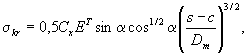
where Cx
is determined according to the graph of Fig. 5.3 depending on the value
of x = D0m/Dm or by the
formula
 at 0
< x < 0.8,
at 0
< x < 0.8,
where a1
= 1.098; a2 = -0.823; a3 = 16.250; a4
= 6.936; a5 = -6.603.
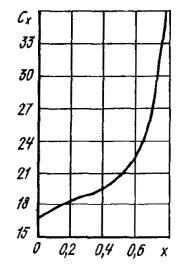
Fig. 5.3
Graphs for determination of coefficient Cx
At the
boundaries of a gap
C0 = 17; C0.8
= 38.
5.5.5.4. Critical
pressure
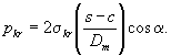
5.5.5.5. Permissible external pressure
[pa]
= 0.5xpkr,
where correction
coefficient
x = min{0.7;
λ/(1 + λ)}, where λ = RTp0.2/σkr.
5.5.5.6. Stability
of the conical adapter is ensured if the condition of item 5.5.1.9.
5.5.6. The conical
adapters are under the axial force.
5.5.6.1. The
formulas are applicable to calculate the smooth conical adapters under the
axial force satisfying the conditions
0.005 ≤ (s - c)/D0m
≤ 0.1; 10 ≤ α ≤ 60°;
0.005 ≤ (s – c)/Dm
≤ 0.1.
5.5.6.2. At α
<10°, a conical adapter can be considered as a cylindrical shell which
length is equal to the cone height, and the mean diameter is equal to the
larger base diameter.
The wall
thickness of the cylindrical shell is assumed to be equal to the wall thickness
of the conical adapter.
5.5.6.3. Design
axial compression stress
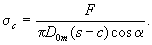
5.5.6.4. Critical
stress
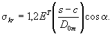
5.5.6.5. Permissible compression
stress
[σc] = 0.5xσkr,
where correction
coefficient
x = min{0.25;
λ/(1 + λ)}, where λ = RTp0.2/σkr.
5.5.6.6. Stability
of the conical adapter is ensured if the condition of item 5.5.2.9.
5.5.7. The
conical adapters under the joint action of external pressure and axial force.
Stability of
the conical adapter is ensured if the condition of item 5.5.3.3 is
followed where the permissible pressure [pa] is determined
according to item 5.5.5, and the design axial compression stress σc
and permissible compression stress [σc] are determined
according to item 5.5.6.
5.5.8. Calculation
for stability under creep conditions.
5.5.8.1. Calculation
for stability under creep conditions involves determining the permissible
operating lifetime when the given external pressure and compression loads
effect on the calculated structural component, or determining the permissible
loads for the specified operating lifetime of equipment.
In the
calculations, the steady-state creep function, which has the following form, is
used
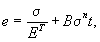
where e is deformation;
σ is rated stress determined according to items 5.5.8.2 - 5.5.8.5,
MPa (kgf/mm2); B is creep coefficient, (1/MPa)n
· s-1 [(mm2/kgf)n · h-1]; n
is creep parameter; t is time, s (h).
Values of B
and n are determined by creep curves on the basis of the dependence
between e and σ given in this item.
The
calculation may be used if σkr < Rp0.2.
5.5.8.2. The
formulas are applicable to calculate smooth long cylindrical components under
the external pressure when satisfying the following condition:
0.005 ≤ (s - c)/Dm
≤ 0.2.
Design
operating lifetime
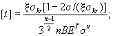
B, n - see in item 5.5.8.1.
Critical
stress
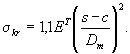
Correction
coefficient x is determined by the formula in item 5.5.1.8.
Rated stress

5.5.8.3. The
formulas are applicable to calculate full and truncated conical shells with an
angle of taper that satisfy the conditions
0.005 ≤ (s - c)/Dm
≤ 0.1; 10 ≤ α ≤ 60°.
Design
operating lifetime
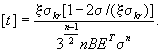
Rated stress
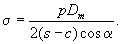
Critical
stress
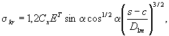
where Cx
is determined according to graph in Fig. 5.3 depending on x = D0m/Dm;
D0m, Dm are mean diameters of
smaller and larger bases of the conical shell, respectively, mm.
Correction
coefficient x is determined by the formula in item 5.5.5.5;
α is an angle of taper equal to half the angle of cone at the apex, degr.
5.5.8.4. The
formulas are applicable to calculate spherical, elliptical, and torospheric
shells which satisfy the condition
0.005 ≤ (s - c)/Dm
≤ 0.1.
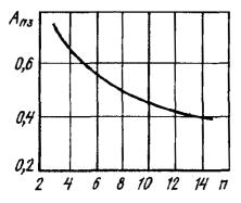
Fig. 5.4.
Graph to determine An3
Design
operating lifetime
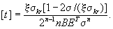
Rated stress
 - for
spherical shells;
- for
spherical shells;
 - for
elliptic and torospheric shells.
- for
elliptic and torospheric shells.
Critical
stress
σkr
= 1.2ЕT(s - c)/Dm – for
spherical shells;
σkr
= 0.6ETb2(s - c)/b12
– for elliptic and torospheric shells;
b1, b2
are major and minor semi-axes of elliptical or torospheric shells,
respectively, mm.
5.5.8.5. The
formulas are applicable to calculate smooth cylindrical shells loaded with
axial compression and satisfying the condition
0.005 ≤ (s - c)/Dm
≤ 0.2.
Design axial
stress
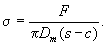
Design
operating lifetime is determined as the smallest of two values:
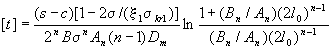
and
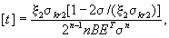
where x1 –
see item 5.5.2.8; σkr1 – see item 5.5.2.6;

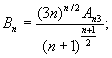
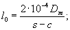 B,
n – see item 5.5.8.1; x2 – see item 5.5.2.8; σkr2
– see item 5.5.2.7; An3 is determined
according to graph in Fig. 5.4 depending on n.
B,
n – see item 5.5.8.1; x2 – see item 5.5.2.8; σkr2
– see item 5.5.2.7; An3 is determined
according to graph in Fig. 5.4 depending on n.
5.5.8.6. The
stability of components of structures will be ensured when the condition t
≤ [t] is followed.
5.6. CALCULATION FOR CYCLIC
STRENGTH
5.6.1. The method
of calculating the cyclic strength is applicable below the temperature Tt
(see Section 3.2 Regulations) for parts made of zirconium alloys from 1
to 2.5% niobium, carbon and alloyed steels, corrosion-resistant steels of
austenitic class, heat-resistant chrome-molybdenum-vanadium steels and
iron-nickel alloys.
5.6.2.
Determination of the permissible number of cycles by given stress amplitudes or
permissible stress amplitudes for a given number of cycles is carried out:
1) according
to design fatigue curves, which characterize, within the limits of their
application, the dependence between the permissible amplitudes of conditional
stresses and the permissible numbers of cycles, or
2) according
to the formulas binding the permissible amplitudes of conditional stresses and
the permissible numbers of cycles, in cases of a refined calculation of
permissible numbers of the cycles or amplitudes of stresses, or when the design
curves cannot be applied.
5.6.3.
Amplitude of the operating stress shall not exceed the permissible amplitude of
stress [σaF], obtained for a given number of cycles N.
If the stress amplitude is set, then the operating number of cycles N
shall not exceed the permissible number of cycles [N0].
If the loading
process consists of a series of cycles characterized by stress amplitudes (σaF)i
and corresponding cycle numbers Ni, then the strength
condition for accumulated fatigue damage shall be met.
5.6.4. For carbon
and alloyed steels in the temperature range from 293 to 623 K (from 20 to 350
°C) with values of RpT0.2/RTm
≤ 0.7; RTm ≥ 450 MPa; ZT ≥ 32 %
and ET = 195 GPa design fatigue curve is shown in Fig. 5.5.
For austenitic
steels in the temperature range from 293 to 723 K (from 20 to 450 °C) with
values of RpT0.2/RTm
≤ 0.7; RTm ≥ 350 MPa; ZT ≥ 45 %
and ET = 173 GPa design fatigue curve is shown in Fig. 5.6.
For carbon and
alloyed steels in the temperature range from 293 to 623 K (from 20 to 350 °C),
values of 0.7 < RpT0.2/RTm
≤ 0.8; RTm ≥ 500 MPa; ZT ≥ 45 %
and ET = 190 GPa design fatigue curves are shown in Fig. 5.7,
and for steels in the temperature range from 293 to 623 K (from 20 to 350 °C)
at values of 0.8 < RpT0.2/RTm
≤ 0.9; RTm ≥ 500 MPa; ZT ≥ 45 %
and ET = 190 GPa design fatigue curves are shown in Fig. 5.8.
Curves in Fig.
5.7 and 5.8 are constructed for different values of the
concentration coefficient of reduced stresses K(σ).
Design curves
in Fig. 5.5 - 5.8 are obtained with due regard to the maximum
safety coefficients. These curves are allowed to be used when the stress cycle
asymmetry coefficients are r ≤ 0.
5.6.5. The
permissible amplitude of conditional elastic stress for given temperatures
below those set in item 5.6.4 can be determined by multiplying the
values of [σaF] according to design curves in Fig. 5.5
- 5.8 by the ratio of the modulus of elasticity at a given temperature
to the modulus of elasticity at the maximum temperature of application of the
corresponding design curve.
5.6.6. The
permissible amplitude of conditional elastic stress or the permissible number of
cycles for steels with the ratio of RpT0.2/RTm
≤ 0.7 at [N0] ≤ 1012 is determined by the formulas
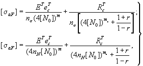 (5.20)
where nσ,
nN are the safety coefficients for stresses and number of
cycles; m, me are material characteristics; r
is a stress cycle asymmetry coefficient; RTc is a
strength characteristic assumed to be equal to
RTc = RTm(1
+ 1.4 · 10-2ZT);
eTc is a
plasticity characteristic depending on the value of ZTc
is determined by the formula
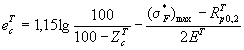 (5.21)
or at (σ*F)max
< RTp0.2 – by the formula
 (5.22)
When using
data of state standards, specifications for the material or data of Appendix 1
Strength Calculation Regulations, which provide guaranteed mechanical
characteristics, when ZT ≤ 50 %, it shall be assumed ZTc
= ZT. When ZT > 50 %, it shall be
assumed ZTc = 50 %.
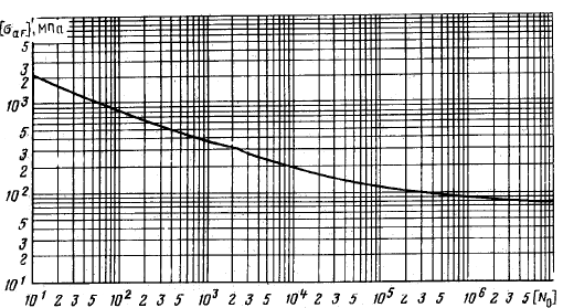
Fig. 5.5.
Design fatigue curve of carbon and alloyed steels with RpT0.2/RTm
≤ 0.7 to T = 623 K (350 °C)
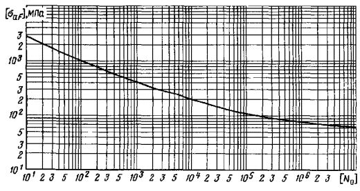
Fig. 5.6.
Design fatigue curve of austenitic steels to M = 723 K (450 °C)
If the
plasticity characteristic eTc is determined
according to the value of ZT formulated in a static tensile
test, the following formulas are used
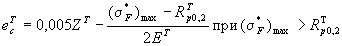 (5.23)
and
eTc = 0.005ZT
at (σ*F)max ≤ RTp0.2.
(5.24)
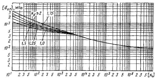
Fig. 5.7.
Design fatigue curves of carbon and alloyed steels with 0.7 < RpT0.2/RTm
≤ 0.8 to
T = 623 K (350 °C)
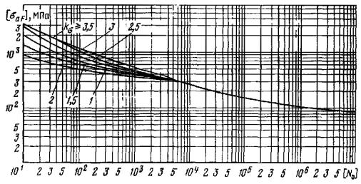
Fig. 5.8.
Design fatigue curve of carbon and alloyed steels with 0.8 < RpT0.2/RTm
≤ 0.9 to
T = 623 K (350 °C)
Characteristics
ET, ZT, RTm
are assumed to be equal to the minimum values in the range of working
temperatures with due regard to aging. Safety coefficient for stresses nσ
= 2, and for number of cycles nN = 10.
When
calculating components which carry only thermal loads (e.g. heat shields and
similar parts) or both thermal and mechanical loads while deformation is
limited by other elastic bearing components (e.g. anti-corrosion body jacket),
and fracture of which shall not lead to coolant exit beyond the bearing
components, safety coefficients for stresses nσ and cycle
number nN are assumed to be equal to 1.5 and 3
correspondingly.
In the
calculation of welded joints with incomplete penetration made by austenitic
electrodes and used in the above parts, with due regard to the effective
concentration coefficient according to item 5.3.10, safety coefficients
are assumed to be equal to nσ = 1.25 and nN
= 2.1.
Exponents m
and me and endurance limit RT-1
are assumed according to Table 5.7.
If the
permissible number of cycles [N0] ≤ 106, then
definition [σaF] is allowed by the formulas
 (5.25)
Of two values
of [N0] or [σaF], determined by the
formulas (5.20) or (5.25), the smallest is selected.
Table 5.7. Exponent
values of m and me and endurance limit values RT-1
|
Designation
|
RTm ≤ 700 MPa
|
700 < RTm
≤ 1200 MPa
|
|
RT-1 (at
symmetrical cycle)
|
0.4RTm
|
(0.54 - 2 ·
10-4RTm)RTm
|
|
m
|
0.5
|
0.36 + 2 ·
10-4RTm
|
|
me
|
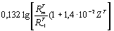
|
5.6.7. The
permissible stress amplitude or the permissible number of cycles for pearlite
steel with values of [N0] ≤ 1012 and RpT0.2/RTm
> 0.7 are determined by the formulas (5.20) or (5.25) and by
the formula
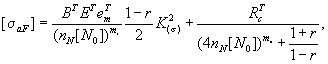 (5.26)
where the safety
coefficient for the number of cycles nN = 10; BT,
m1 are material characteristics. For steels at values of RpT0.2/RTm
≥ 0.7, the value of BT is determined by the formula
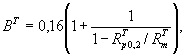 (5.27)
and the exponentm1
is determined by the formula
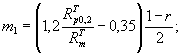 (5.28)
eTm is a
plasticity characteristic characterized by the value of uniform relative
contraction ZmT is determined by the formula
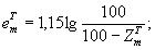 (5.29)
Kσ – theoretical reduced stress
concentration coefficient.
Characteristics
of mechanical properties ET, ZTm,
RTc are assumed to be equal to the minimum values
in the considered range of temperatures with due regard to aging.
For parts
calculated by the formulas (5.20) or (5.25) with reserve
coefficient nσ = 1.5 and nN = 3, safety
coefficient according to the number of cycles when calculating by the formula (5.26)
is assumed to be equal to 3.
The value of
uniform contraction of the cross section (contraction at a stress equal to the
strength limit) is determined experimentally in accordance with the tensile
test method or by the formula
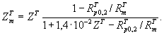 (5.30)
Of three
values of [σaF ] or [N0] generally
determined by the formulas (5.20) or (5.25) and (5.26),
the smallest is selected.
At a number of
cycles [N] = 106, is it allowed to use the following formula
instead of the formula (5.26) in order to determine the permissible
stress amplitude
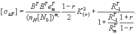
5.6.8. The stress
cycle asymmetry coefficient at
(σF)max
< Rp0.2(Tmin) and 2(σaF)
< [Rp0.2(Tmin) + Rp0.2(Tmax)]
is calculated by the
formula
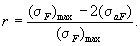 (5.31)
If the cycle
asymmetry coefficient r < -1 or r > 1, then in the
calculation it is assumed r = -1.
At 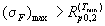 and
and  the cycle
asymmetry coefficient is determined by the formula (5.31), where (σF)max
is replaced by the maximum stress from the elastic plastic calculation. It is
allowed to use the formula
the cycle
asymmetry coefficient is determined by the formula (5.31), where (σF)max
is replaced by the maximum stress from the elastic plastic calculation. It is
allowed to use the formula
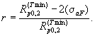 (5.32)
In case of
simultaneous fulfillment of conditions 
 and
and 
asymmetry coefficient r
= -1.
At  the
asymmetry coefficient is determined by the formula
the
asymmetry coefficient is determined by the formula
 (5.33)
If according
to the formulas (5.31) - (5.33) the cycle asymmetry coefficient r
will be between -1 to -1.2, then when calculating the amplitude of stresses by
the formula (5.26) it is assumed r = -1.
5.6.9. Calculation
by the formula (5.26) is not performed if one of the following
conditions is met:
1) the
asymmetry coefficient r < -1.2 or r > 1;
2) stresses
are caused only by the action of a bending moment or by thermal loads at
compression or zero stresses mean in section.
5.6.10. Residual
stress is taken into account if it is tensile and, in the zone under
consideration, the amplitude of the local conditional elastic stress from
mechanical and thermal loads does not exceed the yield limit at a temperature
of 293 K (20 °C) at any type of loading cycle. It is allowed to assume the
residual stress equal to the yield limit at a temperature of 203 K (20 °C).
When determining the permissible stress amplitude by the formula (5.26),
the residual stress is not taken into account.
5.6.11. Residual
stress is taken into account when determining the value of the stress cycle
asymmetry coefficient by algebraically summing it with the stress from
operating mechanical and thermal loads only in the case of calculation by the
design fatigue curves in Fig. 5.5 - 5.8 (in Fig. 5.7, 5.8
only by surface curves) and by the formulas (5.20) and (5.25).
When
determining the asymmetry coefficient in the calculation of non-heat-treated
incomplete-penetration welded joints, the stress (σF)max
is assumed to be equal to the yield limit at the minimum temperature of a
cycle.
5.6.12. Permissible
stress amplitude for welded joint [σaF]s,
with the exemption of incomplete-penetration welded joint (item 5.3.11),
is determined by the formula
[σaF]s
= φs[σaF],
where [σaF]
is an amplitude of permissible conditional elastic stresses, determined by the
design fatigue curve or by the corresponding formula for the base material at a
given number of cycles; φs is a coefficient depending on the
type of welding of welded materials and the heat treatment after welding (φs
≤ 1).
Values of φs
for a number of welded joints are given in Table 5.8. Coefficient φs
is used in conjunction with the design fatigue curve of the base material, in
relation to which φs is determined.
For other
welding methods, welding and welded materials that are not listed in Table 5.8,
the value of φs is determined experimentally.
In the absence
of data on the value of φs data of Table 5.9 may be
used.
5.6.13. When
calculating bodies with anti-corrosion deposit welding, the assessment of
cyclic strength is carried out separately for the base metal and the deposit
welding metal by the curves and calculation formulas of this section, with due
regard to coefficient φs.
Coefficient φs
for the body deposit welding is used in conjunction with the design fatigue
curve of the base metal of body according to item 5.6.6.
The value of φs
for manual welding of austenitic steel with electrodes grades EA-395/9 and
EA-400/10U can be used in calculating a heterogeneous welded joint of pearlite
steels with austenitic steel for the layer welded over pearlite steel using the
design fatigue curve of austenitic steel.
5.6.14. For
threaded sections of pins and bolts of pearlite steel at temperatures 293 to
623 K (20 to 350 °C), design fatigue curves (Fig. 5.9, 5.10) are
used, taken with due regard to safety coefficients nσ = 1.5
and nN = 5.
Design curves
in Fig. 5.9 are applied at values of 650 ≤ RTm
< 750 MPa; ZT ≥50 % and ET = 190 GPa.
Design curves
in Fig. 5.10 are applied at values of RTm ≥
750 MPa; ZT ≥ 40 % and ET = 190 GPa.
5.6.15. Specified
calculation of threaded sections of pins and bolts is carried out in accordance
with item 5.3.8 and formulas (5.20) or (5.25). In this
case, the safety coefficients nσ and nN are
assumed to be equal to 1.5 and 3, respectively. When using the concentration
coefficients Kef, the safety coefficients nσ
and nN are assumed to be equal to 1.5 and 5, respectively.
Table 5.8.
Cyclic strength reduction coefficients of welded joints
|
Base metal
|
Welding
technique
|
Welding
material
|
Types of
heat treatment after welding
|
φs
|
|
Steels grades 20, 22K,
20K
|
Manual
|
Electrode of
UONI-13/45 grades
UONI-13/45A
|
Without heat
treatment; tempering; normalization and tempering
|
1.0
|
|
Electrode of
UONI-13/55 grades
|
Without heat
treatment; tempering of up to 10 h
|
φs =
0.8 at (σ(aF)) > 400 MPa; φs = 1.46 -
0.26lg(σ(aF)) at 60 < (σ(aF)) ≤
400 MPa; φs = 1.0 at (σ(aF)) ≤ 60 MPa
|
|
Tempering of more than
15 h
|
1.0
|
|
Automatic submerged
|
Welding wire of grade
Sv-08A
Sv-08GSMT
EP-458
|
Without heat treatment
|
0.9
|
|
Tempering
|
1.0
|
|
Electroslag
|
Welding wire of grade
Sv-10G2
Sv-08GSMT
|
Normalization and
tempering; quenching and tempering
|
1.0
|
|
Steels grades
12Kh2MFA, 15Kh2MFA, 15Kh2MFA-A
|
Manual
|
Electrodes grades N-3,
N-6, N-10
|
Tempering
|
1.0
|
|
Automatic submerged
|
Welding wire grade
Sv-10KhMFT; Sv-10KhMFTU
|
"
|
φs =
0.8 at (σ(aF)) > 500 MPa; φs = 1.34 -
0.24lg(σ(aF)) at 70 < (σ(aF)) ≤
500 MPa; φs = 0.9 at (σ(aF)) ≤ 70 MPa
|
|
Electroslag
|
Welding wire of grade
Sv-13Kh2MFT
|
Quenching and
tempering
|
0.8
|
|
Submerged automatic
strip overlay welding
|
Electrodes grades
Sv-07Kh25N13, Sv-08Kh19N10G2B
|
Tempering
|
0.8
|
|
Manual electrode
overlay welding
|
Electrodes grades
EIO-8, EA-898/21B
|
Tempering
|
0.8
|
|
Steels grades
15Kh2NMFA, 15Kh3NMFA, 15Kh2NMFA-A, 15Kh3NMFA-A
|
Manual
|
Electrode of N-23
grade
|
"
|
1.0
|
|
Automatic submerged
|
Welding wire grade
Sv-08KhGNMTA
|
"
|
1.0
|
|
Electroslag
|
Welding wire grade
Sv-16Kh2NMFTA
|
Quenching and
tempering
|
1.0
|
|
Austenitic steels
|
Manual
|
Electrode of EA-395/9
grade
|
Without heat treatment
|
1.0
|
|
Electrodes grades
EA-400-10U, EA-898/21B, EIO-8
|
Tempering
|
0.8
|
|
Argonarc
|
Welding wire of grade
Sv-04Kh19N11M3
|
Without heat
treatment, tempering
|
1.0
|
Table 5.9. Values
of the cyclic strength reduction coefficient for the welded joint
|
Base
material (steel)
|
φs
for welded joint
|
|
after
tempering
|
without
tempering
|
|
Carbon,
silicon-manganese, alloyed, RTm ≤ 380 MPa
|
0.75
|
0.75
|
|
Alloyed, 380 < RTm
≤ 520 MPa
|
0.70
|
0.65
|
|
Alloyed, 520 < RTm
≤ 700 MPa
|
0.60
|
0.50
|
|
Austenitic
|
0.70
|
0.60
|
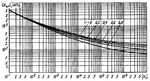
Fig. 5.9.
Design fatigue curves for threaded sections of pins and bolts of pearlite
steels from
650 ≤ RTm < 750 MPa to T = 623 K (350
°C) at different values of asymmetry coefficient r
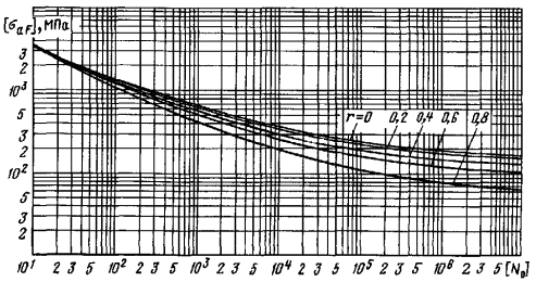
Fig.
5.10. Design fatigue curves for threaded sections of pins and bolts of pearlite
steels from RTm ≥ 750 MPa to T =
623 K (350 °C) at different values of asymmetry coefficient r
Cycle
asymmetry coefficient of local stresses is determined by the formulas (5.31)
- (5.33).
5.6.16. In cases
where low-frequency cyclic stresses associated with starting-up, shutdown,
power change, actuation of emergency protection, or other modes, are
accompanied by the imposition of high-frequency stresses, such as those caused
by vibration, temperature pulsation when mixing coolant flows with different
temperatures, the cyclic strength is calculated with due regard to
high-frequency loading.
5.6.17. Input data
on high-frequency loading is obtained by analyzing the results of measurements
during the operation of a component of structure or by their calculation.
5.6.18. In the
calculation of the permissible number of cycles under high-frequency loading,
only fatigue curves are used, obtained by the formulas (5.20), (5.25),
for steels with an ratio both like RTp0.2/RTm
≤ 0.7 and RTp0.2/RTm
> 0.7.
5.6.19. The
strength condition in the presence of various cyclic loads is checked by the
formula
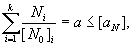 (5.34)
where Ni
is a number of cycles of the i-th type during operation time; k
is a total number of cycle types; [N0]I is a permissible
number of cycles of i-th type; a is a cumulative fatigue damage
which limit value is [aN] = 1.
In general
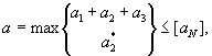 (5.35)
where a1
is damage from operational loading cycles to which high-frequency stresses are
not imposed; a2 are damages from high-frequency stresses at
constant operating stresses (steady-state modes); a*2
is damage of a2 type determined for loading conditions in
steady-state modes resulting in the greatest damage over the entire operation
time; a3 is the amount of damages from high-frequency
stresses during cycles of alternating stresses in transient operating
conditions a*3 and with the passage of resonant
frequencies a**3 in the same cycles.
Accumulated
damage a1 and a2 are determined by the formula (5.34).
Amplitude and frequency values for detection of damages a2
and a3 are assumed in accordance with Section 6.3 of
Appendix 8.
5.6.20. Combination
of main cyclic loading with amplitude (σaF) and frequency f0
and imposed with amplitude <σa> and frequency f
causes a decrease in the permissible number of cycles of the main low-frequency
loading from [N0 ] to [N], determined by the formula
[N] = [N0]/χ,
(5.36)
where χ is a durability
reduction coefficient when applying high-frequency cycles used in determining
damage a*3.
For the main
loading cycle of the i-th type, the damage a*3 is
determined by the formula
(a*3)i
= χiNi/[N0]i.
(5.37)
The
coefficient χ, irrespective of the degree of stress concentration, residual
stresses, cycle asymmetry, value of nominal stresses and temperature, is
determined by the nomograms shown in Fig. 5.11 and 5.12, or
calculated by the formula
 (5.38)
where f0
= 1/(t1 + t2) is a frequency of the main
cycle of alternating stresses, determined without taking into account the
period of time during which the additional stresses are
applied to the constant ones (Fig. 5.13); (σa) is
an amplitude of the reduced stresses of the main cycle without stress
concentration; η is a coefficient depending on the material, taken according to
Table 5.10.
In the absence
of experimental data for preliminary assessment, the value of η is assumed to
be equal to 2.
5.6.21. The calculation
method for two-frequency cyclic loading is applicable when all the following
conditions are met:
1) ratio of
the stress amplitude <σa> to the stress amplitude (σa)
is in the interval of
0
< <σa>/(σa)
≤ 0.5; (5.39)
2) the
absolute value of maximum and minimum stresses under two-frequency loading does
not exceed the value of (0.2 · 10-2ET + RTp0.2)
at rated temperature;
3) the ratio f/f0
does not exceed 5 · 106;
4) the number
of cycles with amplitude <σa> within the time t1
+ t2 exceeds 10 (Fig. 5.13).
5.6.22. When
calculating the cyclic strength of parts subjected to exposure, a decrease in
the relative contraction is taken into account. The increase in temporary
resistance due to exposure is not taken into account. Under the effect of
exposure, it is allowed to apply the cyclic strength reduction coefficients
given in Appendix 7.
Table 5.10. Value
of coefficient η
|
Material
type
|
Carbon
steel, RTm ≤ 500 MPa
|
Austenitic
steel, RTm ≤ 550 MPa
|
Alloyed
steel, 500 < RTm ≤ 800 MPa
|
Alloyed
steel, RTm > 800 MPa
|
|
η
|
1.3
|
1.54
|
1.8
|
1.9
|
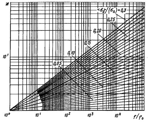
Fig. 5.11.
Values of χ for pearlite steels and their welded joints with RTm
≤ 500 MPa
5.6.23. If, when
calculating the cyclic strength of a component of structure, the required
safety coefficients are not met, then the cyclic strength is assessed on the
basis of experimental fatigue curves obtained in accordance with the fatigue
test method (Appendix 2) for the considering loading conditions and
state of structure metal, with due regard to the corresponding safety
coefficients nσ and nN or according to the
results of tests of full-size components or their models, designed and manufactured
in accordance with the requirements for regular structures.
The
geometrical similarity of the models shall be ensured, at least in the zone of
verification of the cyclic strength and in the adjacent areas, which influence
the value and distribution of stresses in the tested zone. It is not
recommended to use simulation of a welded joint with a reduction in full-size
dimensions of components and anti-corrosion deposit welding with a change in
its thickness if the purpose of the test is to check their strength.
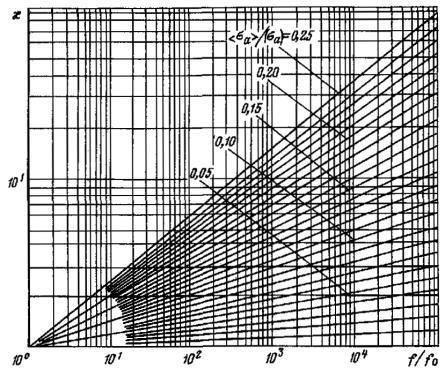
Fig. 5.12.
Values and for austenitic steels and their welded joints with RTm
≤ 550 MPa
The test mode
for the nature of changes in loads and temperatures shall comply with the
operating conditions.
The safety
coefficients are assumed according to the value of the reduced local
conditional elastic stress in the zone that determines durability, or according
to the number of loading cycles, or according to the stress and number of
cycles at the same time.
Safety
coefficients for the conventional stress and number of cycles N ≤ 104
are determined by the formulas
nσ = 1.45 -
0.02x; (5.40)
nN = 3.5 - 0.14x,
(5.41)
where x is a
number of tested objects.
At the same
time, the margins of nσ and nN for the
moment of crack formation under cyclic loading of full-size components of structure
or their models shall not be less than 1.25 and 2.1, respectively.
The conditions
of low- and multi-cycle tests for stresses and number of cycles with
simultaneous use of safety coefficients nσ and nN
are determined using the design fatigue curve for the base metal or welded
joint with the corresponding loading cycle asymmetry and temperature. To do
this, determine the slope m0 of the design fatigue curve at
point with [N0] = Ne, where Ne
is a set number of cycles during operation. The section connecting the points
with coordinates {Ne, nσ(σaF)}
and {(nσ)1/m0Ne, (σaF)}
is a combination of equivalent test modes.
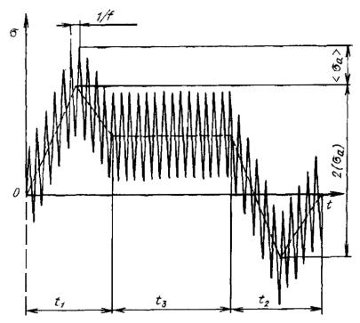
Fig. 5.13.
Cycle form under two-frequency loading
When testing
geometrically similar models, the safety coefficient for reduced local
conditional elastic stress is determined by the formula
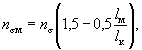 (5.42)
where lm,
lk are linear dimensions of the model and full-size structure
in the tested zone.
Safety
coefficient by the number of cycles when testing the model
 (5.43)
The results of
tests on cyclic strength cannot serve as a ground for increasing the
permissible values of the stress categories used in the calculation of static
strength.
5.6.24. Appendix 12
(recommended) gives a simplified method for calculating the cyclic strength,
which can be used instead of the method in Sections 5.3 and 5.6.
5.7. CALCULATION FOR
LONG-TERM CYCLIC STRENGTH
5.7.1. Long-term
cyclic strength is calculated in relation to the components of structure
operating at temperatures that cause creep and loaded with repeated thermal or
mechanical forces.
5.7.2. The recommended
method for calculating the long-term cyclic strength is given in Appendix 7.
The
calculation uses the characteristics of long-term strength and ductility
according to Tables P6.1 and P6.3.
5.7.3. The
component of structure, calculated on the long-term cyclic strength, shall
satisfy:
1) the
strength conditions taken when selecting the basic dimensions in the entire
range of operating temperatures;
2) the
strength conditions when calculating the long-term static strength.
5.7.4. The use of
other methods is allowed provided that their proper computational-experimental
justification for the materials used and operating conditions and operating
life for the number of cycles and duration of loading.
5.8. CALCULATION FOR
RESISTANCE TO BRITTLE FRACTURE
5.8.1. General.
5.8.1.1. Based on
the provisions of this Section, the resistance to brittle fracture of the NPI
equipment and pipelines shall be calculated at the design stage.
5.8.1.2. Provisions
of this Section shall not be applied to the calculation of fastening parts.
5.8.1.3. Calculation
for the resistance to brittle fracture of equipment and pipeline components is
carried out for all operation modes, including normal operation (NO), abnormal
operation (AO), emergencies, hydraulic (pneumatic) tests.
5.8.1.4. The main
material characteristics used in the calculation are the critical stress
intensity coefficient K1c, critical brittle
temperature Tk and yield limit RTp0.2.
Changes in the
properties of materials during operation are taken into account by introducing
into the calculation of critical brittle temperature shifts due to various
effects during operation.
5.8.1.5. If the wall
thickness of the calculated components is less than the thickness required to
determine the values of K1c in accordance with the
provisions of GOST 25.506-85, it is allowed to use the critical crack opening δc
or other characteristics (Kc, Jc),
determined in accordance with the aforementioned GOST, when calculating the
resistance to brittle fracture.
Procedures of
calculation using these characteristics shall be agreed with the leading
organization for development of strength calculation regulations.
5.8.1.6. Resistance
to brittle failure is deemed ensured if the following condition is complied
with for the selected model defect in the form of a crack in the analyzed
operating mode
K1 ≤ [K1]i,
where [KI
]i is the permissible value of the stress intensity
coefficient.
The index i
means that the permissible values of the stress intensity coefficients are
selected different depending on the design conditions:
i = 1 - for
normal operation; i = 2 - for hydraulic (pneumatic) tests and abnormal
operation; i = 3 - for emergency.
5.8.1.7. When
determining [KI]i, the value of transfer of
neutrons Fn and temperature T are assumed to be equal
to their values at the point corresponding to the greatest depth of the
selected design crack.
5.8.1.8. If at the
time of enforcement of these regulations it is necessary to carry out
calculations of equipment and pipelines in operation, manufacture or
installation, or completed by the detailed design, it is allowed:
1) to use the
provisions of this calculation;
2) for
equipment and pipelines in operation, by agreement between the design
(engineering) organization, lead material organization, enterprise owning the
equipment and pipelines, to determine the parameters of defects allowed under
the terms of ensuring strength, and by control to confirm the absence of
equipment and pipelines defects parameters of which exceed the permissible by
calculation; the calculation shall use the actual material properties, and the
calculation itself (including the schematization of defects revealed during the
control process) shall be carried out according to the procedures agreed with
the leading organization for development of strength calculation regulations;
3) for
equipment and pipelines in manufacture, installation, or completed by the
detailed design, it is allowed to use procedures that differ from those
described in this Section by agreement with the leading organization for
development of strength calculation regulations and the USSR
Gosatomenergonadzor.
5.8.1.9. It is
allowed not to carry out brittle fracture resistance calculation for components
of structure that are not exposed to neutron exposure (or exposed at
temperatures of 250-350 °C before transfer of no more than 1022
neutrons/m2 at E ≥ 0.5 MeV) in the following cases:
1) the
components of structure are made of corrosion-resistant steels of austenitic
class or non-ferrous alloys;
2) materials
of the components of structure (including welded joints) have a yield limit at
a temperature of 20 °С less than 300 MPa (30 kgf/mm2), and the wall
thickness of the component of structure is not more than 25 mm;
3) materials
of the components of structure (including welded joints) have a yield limit at
a temperature of 20 °С less than 600 MPa (60 kgf/mm2), and the wall
thickness of the component of structure is not more than 16 mm;
4) wall
thickness of the considered component of structure s, mm, satisfies the
condition
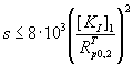
at [KI]1
in MPa · m1/2 and RTp0.2 in
MPa (both characteristics are assumed at the lowest operation temperature and
critical brittleness temperature Tk, corresponding to the end
of operation).
5.8.1.10. Thickness
of an anti-corrosion coating is not included in the calculated wall thickness
of the components of equipment and pipelines.
5.8.2. Stress
intensity coefficient.
5.8.2.1. The stress
intensity coefficient for the selected design cracks is determined
analytically, numerically or experimentally according to procedures agreed with
the leading organization for development of strength calculation regulations.
5.8.2.2. The stress
intensity coefficient, MPa · m1/2, for cylindrical, spherical,
conical, elliptical, ans flat components loaded with internal pressure and
temperature effects, can be determined by the formula
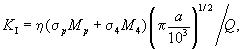
where η is a coefficient
taking into account the effect of stress concentration; σp is
a tensile stress component, MPa; σ4 is a bending stress component,
MPa; Mp = 1 + 0.12(1 - a/c); Mq
= 1 - 0.64a/h; a is a crack depth, mm; c is a half
length of crack, mm; h is a length of the zone within which the bending
stress component retains its positive value, mm;
Q = [1 + 4.6(a/2c)1.65]1/2.
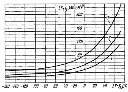
Fig. 5.14.
Steels grades 12Kh2MFA, 15Kh2MFA, 15Kh2MFA-A:
1 - NO,  2
- AO and hydraulic (pneumatic) tests,
2
- AO and hydraulic (pneumatic) tests,  3 -
emergency,
3 -
emergency, 
The formula is
valid when a ≤ 0.25s and a/c ≤ 2/3, where s
is a product wall thickness.
When
calculating zones where there is no stress concentration, it is assumed that η
= 1.
5.8.2.3. The
component of (ring or axial) tension stresses is determined by the formula

where j is θ coordinate
or Z; σj is a stress variation function for wall
thickness; s is a wall thickness in the design section.
5.8.2.4. The value
of the component of bending stress is determined by the formula
σjq
= σjn – σjp,
where σjn
is a value of the function of stress variation across the wall thickness at the
point n.
For components
without anti-corrosion deposit welding, point n is placed on the outer
or inner surface of the product in the zone of maximum tension stresses. For
components with anti-corrosion deposit welding, point n is selected on
the outer surface of the product or on the interface between the anti-corrosion
coating and base metal in the zone of tension stresses.
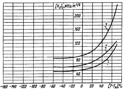
Fig. 5.15.
Steels grades 15Kh2NMFA, 15Kh2NMFA-A:
1 - NO,  2 - AO and hydraulic (pneumatic) tests,
  3 - emergency,
5.8.3. Permissible
values of stress intensity coefficients.
5.8.3.1. Permissible
values of stress intensity coefficients depend on the reduced temperature (T
– Tk) and design case. Dependence [KI]i
on [T - Tk ] is taken as the envelope of two curves
determined by the initial temperature dependence KIc.
One of these curves is obtained by dividing the ordinates of the initial curve
by the safety coefficient nk, and the other – by shifting the
original curve along the abscissa by the value of the temperature margin ∆T.
The following
values are assumed:
for normal operation (i
= 1) nk = 2, ∆T = 30 °C;
when abnormal operation
and hydraulic (pneumatic) tests (i = 2) nk = 1.5, ∆T
= 30 °C;
for emergencies (i
= 3) nk = 1, ∆T = 0 °C.
5.8.3.2. Initial
temperature dependences K1c are assumed according to
the data given in the relevant qualification reports for materials (base metal,
welded joints), or according to the engineering solutions agreed with the USSR
Gosatomenergonadzor, lead material organization, and lead organization for
development of strength calculation regulations.
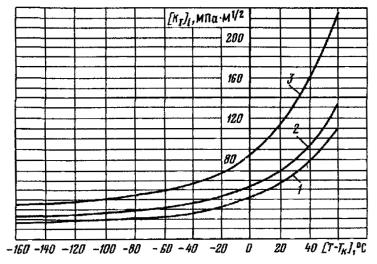
Fig. 5.16.
Welded joints of steels grades 15Kh2MFA, 15Kh2MFA-A, 15Kh2NMFA, 15Kh2NMFA-A:
1 - NO,  2
- AO and hydraulic (pneumatic) tests,
2
- AO and hydraulic (pneumatic) tests, 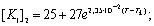 3 - emergency,

5.8.3.3. Temperature
dependencies [KI]i for steels of 12Kh2MFA,
15Kh2MFA, 15Kh2MFA-A, 15Kh2NMFA, 15Kh2NMFA-A grades and their welded joints are
shown in Fig. 5.14 – 5.16.
5.8.3.4. For
pearlite steels and high-chromium steels and their welded joints with a yield
limit at a temperature of 20 °C, established according to the instructions of
item 3.7 hereof and not exceeding 600 MPa (60 kgf/mm2),
generalized curves of permissible stress intensity coefficients given in Fig. 5.17
may be used.
5.8.4.
Critical brittle temperature.
5.8.4.1. Critical
brittle temperature of a material is determined by the formula.
Tk = Tk0
+ ∆TT + ∆TN + ∆TF,
where Tk0
is a critical brittle temperature of a material in the initial state; ∆TT
is a shift of the critical brittle temperature due to temperature aging; ∆TN
is a shift of the critical brittle temperature due to cyclic damage; ∆TF
is a shift of the critical brittle temperature due to the influence of neutron
exposure.
5.8.4.2. Values of Tk0,
∆TT, ∆TN, ∆TF (or
coefficient of radiation embrittlement AF) are assumed
according to the data given in the relevant qualification reports for materials
(base metal, welded joints), or according to the engineering solutions agreed
with the USSR Gosatomenergonadzor, lead material organization, and lead
organization for development of strength calculation regulations.
Fig. 5.17.
Generalized dependencies of permissible stress intensity coefficients:
1 - NO,  2 - AO and hydraulic (pneumatic) tests,
  3 - emergency,
Procedures for
determining values of Tk0, ∆TT, ∆TN,
∆TF (or AF) are given in Appendix 2.
5.8.4.3. It is
allowed to use values of Tk0, ∆TT,
AF, given in Table 5.11.
5.8.4.4. It is
allowed to determine values of ∆TN by the formula
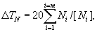
where Ni
is a number of loading cycles at the i-th operation mode; [Ni]
is a permissible number of cycles for the i-th operation mode; m
is a number of modes.
5.8.4.5. It is
allowed to determine values of ∆TF by the formula
∆TF = AF(Fn/F0)1/3,
where AF
is a radiation embrittlement coefficient, °C; Fn is a neutron
transfer with E ≥ 0.5 MeV, neutron/m2; F0 =
1022 neutron/m2.
The formula is
valid when
1022 ≤ Fn
≤ 3 · 1024 neutron/m2.
The values of AF
is assumed according to the documentation data of item 5.8.4.2 and Table
5.11.
5.8.4.6. In the
calculation of components of structures made of steels of 12Kh2MFA, 15Kh2MFA,
15Kh2MFA-A, 15Kh2NMFA, 15Kh2NMFA-A grades and their welded joints subjected to
neutron exposure at Fn ≥ 1022 neutron/m2
(E ≥ 0.5 MeV) at temperatures 250 - 350 °C, it is assumed that ∆TT
= 0.
Table 5.11. Values
of fracture resistance characteristics
|
Grade
of basic material
|
Type of
welding, grade of welding material
|
Standard
or technical specifications
|
Tk0, °C
|
∆TT,
°C (see
Note 1)
|
Exposure
temperature, °C
|
AF, °C (see
Note 2)
|
|
15Kh2MFA
|
-
|
TU 5.961-11060-77,
Not. 6-90-3315
|
0
|
0
|
250
270
290
|
22
18
14
|
|
15Kh2MFA-A
|
-
|
TU 108.131-75, Not.
479
|
0
|
0
|
270
290
|
12
9
|
|
15Kh2NMFA
|
-
|
TU 108.765-78, Not.
4-83
|
0
|
0
|
290 ± 15
|
29
|
|
15Kh2NMFA-A
|
-
|
TU 108.765-78, Not.
4-83
|
-25
|
0
|
290 ± 15
|
23
|
|
15Kh3NMFA
|
|
TU 24-3-15-223-75,
Not. 480,
TU 5.961-11021-79,
Not. 6-90-3305
|
-10
|
0
|
-
|
-
|
|
10KhN1M
|
-
|
TU 14-1-2587-78
|
10
|
10
|
-
|
-
|
|
22К
|
-
|
TU 108-11-543-80
|
40
|
30
|
-
|
-
|
|
10GN2MFA
|
-
|
TU 108.766-78
|
15
|
10
|
-
|
-
|
|
15Kh2NMFA
|
EW, wire Sv-16Kh2NMFTA
|
TU 14-1-3633-83
|
20
|
0
|
-
|
-
|
|
Flux OF-6
|
-
|
|
MAW, electrodes
RT-45A, RT-45AA, RT-45B
|
OST 108.948.01-80
|
0
|
0
|
-
|
-
|
|
15Kh2NMFA-A
|
AAW, wire
Sv-12Kh2N2MAA (including vacuum-induction, vacuum-arc)
|
TU 14-1-2502-78
|
0
|
0
|
290 ± 15
|
20
|
|
Flux FTs-16A
|
TU 108.949-80
|
|
Wire Sv-08KhGNMTA-VI
|
TU 14-1-3675-83
|
0
|
0
|
290 ± 15
|
20
|
|
Flux KF-30
|
TU 5.965-11090-80
|
|
MAW, electrodes
RT-45AA, RT-45B
|
OST 108.948.01-80
|
0
|
0
|
290 ± 15
|
20
|
|
15Kh3NMFA-A
|
AAW, wire
Sv-08KhGNMTA-VI
|
TU 14-1-3675-83
|
0
|
0
|
-
|
-
|
|
Flux KF-30
|
TU 5.965-11090-80
|
|
MAW, electrodes RT-45B
|
-
|
0
|
0
|
-
|
-
|
|
EW, wire Sv-16Kh2NMFTA
|
TU 14-1-3633-83
|
20
|
0
|
-
|
|
|
Flux OF-6
|
-
|
|
15Kh2MFA
|
AAW (see Note 3), wire
Sv-10KhMFT, Sv-10KhMFTU
|
GOST 2246-70
|
40
|
0
|
250
270
|
See Note 2
|
|
Fluxes AN-42, AN-42M
|
-
|
|
|
|
|
|
KF-30
|
TU 5.965-1190-80
|
|
|
|
|
|
EW (see Note 3), wire
Sv-13Kh2MFT
|
GOST 2246-70
|
40
|
0
|
-
|
-
|
|
Flux OF-6
|
-
|
|
|
|
|
|
MAW (see Note 2),
electrodes N-3, N-6
|
TU 5.965-4052-73 .....
|
20
|
0
|
-
|
-
|
|
15Kh2MFA-A
|
AAW (see Note 3),
Sv-10KhMFTU
|
TU 14-1-3034-80
|
20
|
0
|
270
|
15
|
|
Flux KF-30, AN-42M
|
TU 5.965-11090-80
|
290
|
12
|
|
MAW (see Note 2),
electrodes N-3, N-6
|
TU 5.965-4052-73
|
20
|
0
|
270
290
|
15
12
|
|
15Kh2NMFA
|
AAW (see Note 3), wire
Sv-12Kh2NMFA, Sv-12Kh2NMFA-A (including vacuum-induction, vacuum-arc)
|
TU 14-1-2502-78
|
0
|
0
|
-
|
-
|
|
Flux FTs-16, FTs-16A
|
TU 108.949-80
|
0
|
0
|
-
|
-
|
|
Wire Sv-08KhGNMTA
|
TU 14-1-3675-83
|
0
|
0
|
-
|
-
|
|
Flux KF-30
|
TU 5.965-11090-80
|
|
15Kh3NMFA-A
|
AAW, wire
Sv-08KhGNMTA-VI
|
TU 14-1-3675-83
|
0
|
0
|
-
|
-
|
|
Flux KF-3S
|
TU 5.965-11090-78
|
|
MAW, electrodes RT-5B
|
-
|
0
|
0
|
-
|
-
|
|
EW, wire Sv-16Kh2NMFTA
|
TU 14-130-168-75
|
20
|
0
|
-
|
-
|
|
Flux OF-6
|
-
|
|
10KhN1M
|
AAW, wire Sv-10NMA
|
GOST 2246-70
|
10
|
0
|
-
|
-
|
|
Flux AN-42, AN-42M
|
-
|
|
|
|
|
|
Flux KF-31
|
-
|
|
|
|
|
|
Wire Sv-08KhNM
|
GOST 2246-70
|
10
|
0
|
-
|
-
|
|
Flux KF-31
|
-
|
|
|
|
|
|
MAW, electrodes
UONII-13/45A, UONII-13/55
|
-
|
20
|
20
|
-
|
-
|
|
Electrodes N-25
|
-
|
0
|
0
|
-
|
-
|
|
10KhN1M (VK-1A)
|
AAW, wire Sv-10NMA
|
GOST 2246-70
|
0
|
0
|
-
|
|
|
Flux AN-42, AN-42M
|
-
|
|
|
|
|
|
Flux KF-31
|
-
|
|
|
|
|
|
Wire Sv-08KhNM
|
GOST 2246-70
|
0
|
0
|
-
|
-
|
|
Flux KF-31
|
|
|
MAW, electrodes N-25
|
-
|
0
|
0
|
-
|
-
|
|
22К
|
AAW, wire Sv-06A
|
TU 14-1-1569-75
|
0
|
0
|
-
|
-
|
|
Fluxes AN-42, AN-42M
|
-
|
|
|
|
|
|
Wire Sv-08GSMT,
Sv-10GSMT
|
GOST 2246-70
|
40
|
20
|
-
|
-
|
|
Flux AN-42
|
-
|
|
|
|
|
|
Wire Sv-08GS
|
GOST 2246-70
|
15
|
30
|
-
|
-
|
|
Flux FTs-16
|
TU 108.949-80
|
|
|
|
|
|
Wire Sv-08GSMT,
Sv-08GS
|
GOST 2246-70
|
0
|
0
|
-
|
-
|
|
Flux KF-30
|
TU 5.965-11090-78
|
|
MAW, electrodes
UONII-13/45, UONII-13/45A, UONII-13/55
|
-
|
20
|
20
|
-
|
-
|
|
EW, wire Sv-10G2
|
GOST 2246-70
|
40
|
20
|
-
|
-
|
|
Flux AN-8M
|
GOST 9087-81
|
|
|
|
|
|
10GN2MFA
|
AAW, wire Sv-10GNMA
|
TU 14-1-2860-79
|
15
|
10
|
-
|
-
|
|
Sv-10GN1MA
|
TU 14-1-2860-79
|
|
Flux AN-17M
|
GOST 9087-81
|
|
FTs-16
|
TU 108.949-80
|
|
MAW, electrodes PT-30
|
OST 108.948.01-80
|
15
|
10
|
-
|
-
|
|
EW, wire Sv-10GSHMFA
|
TU 14-1-2860-79
|
15
|
10
|
-
|
-
|
|
Flux OF-6
|
-
|
Notes: 1. The
values of ∆TT are given for temperatures of up to 350 °C.
2. The values
of AF are determined from ratios of AF =
800(P + 0.07Cu) at exposure temperature of 270 °C, AF
= 800(Р + 0.07Cu) + 8 at exposure temperature of 250 °C, where P and Cu
are content of phosphorus and copper, %.
3. AAW -
submerged automatic arc welding; MAW - manual arc welding; EW - electroslag
welding.
5.8.5. Calculation
under normal operation.
5.8.5.1. Resistance
to brittle fracture shall be considered secured if the following condition is
met
KI ≤ [KI]1.
5.8.5.2. When
determining KI, a surface semi-elliptical crack with a depth
of a = 0.25s with ratio of a/c = 2/3 is assumed as
a design defect.
5.8.5.3. Size of h
is assumed to be equal to 0.5s.
5.8.5.4. With due
regard to the instructions of items 5.8.5.2 and 5.8.5.3,
we obtain
KI = η(0.7σp
+ 0.45σq)(s/103)1/2, where
σр
and σq in MPa; s in mm; KI in MPa ·
m1/2.
5.8.5.5. Coefficient
η for zones of stiffness transition (connection of flanges with a cylindrical
part of a body, fillets, etc.) is determined by the formulas:
at 0 < s/R2
≤ 5
η = 1 + (Kσ
- 1)0.7 · 1.8/(s/R2);
at s/R2
> 5
η = 1 + (Kσ
- 1)0.7 · 9/(s/R2).
At η > Kσ
it is assumed that η = Kσ.
It is allowed
to determine η according to the graphs in Fig. 5.18.
In formulas, R2
is a radius of concentrator curvature in the design section; Kσ
is a theoretical concentration coefficient (allowed to be assumed equal to the
value of Kσ when tension).
5.8.5.6. Coefficient
η for the zones of holes (connection of branch pipes, nozzles, pipes) is
determined by the formulas:
at s/R ≤
0.8
η = [1 + 5(Kσ
- 1)exp(-0.86s/R1)]1/2;
at s/R
> 0.8
η = [1 + 2(Kσ
- 1)(s/R1)]1/2,
where R1
is a hole radius.
It is allowed
to determine η by the graphs in Fig. 5.19.
5.8.5.7. The
calculation is required to be carried out only up to the given temperature [T
– Tk]*, the largest value of which on the graph is
[KI]1 = f[T - Tk]
and it corresponds to the value of [KI]*1
determined by the formula
[KI]*1
= 0.35RTp0.2(s/103)1/2,
where RTp0.2
in MPa; s in mm, [KI]*1 in MPa ·
m1/2.
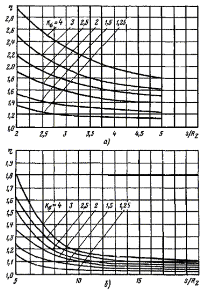
Fig. 5.18.
Dependence of coefficient η on the ratio of s/R2 for
the zones of transition stiffness:
a – 2 ≤
s/R2 ≤ 5; b - s/R2
>5
5.8.6.
Determination of the minimum permissible temperature of the structure during
hydraulic (pneumatic) tests.
5.8.6.1. Hydraulic
(pneumatic) tests shall be carried out in such conditions that the minimum
temperature of the structure during hydraulic (pneumatic) tests Th
is greater than or equal to the minimum permissible temperature of the
structure [Th], determined based on the brittle fracture
resistance calculation.
5.8.6.2. Temperature
[Th] is determined using the condition
KIh ≤ [KI]2,
where KIh
is a stress intensity coefficient in the considered sections of the structure
during hydraulic (pneumatic) tests.
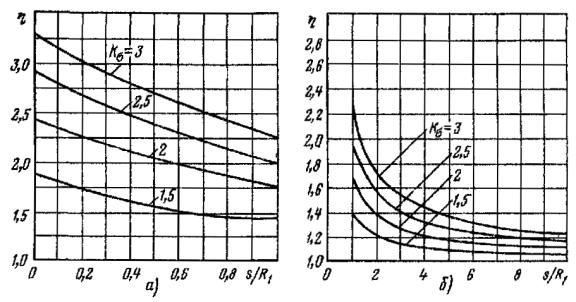
Fig. 5.19.
Dependence of coefficient η on the ratio of s/R1 for
the zones of holes:
a - s/R1
≤ 1; b - s/R1 > 1
5.8.6.3. The values
of KIh is determined in accordance with the
instructions of items 5.8.2, 5.8.5.2 and 5.8.5.3.
5.8.6.4. The value
of [KI]2 is assumed to be equal to the value of KIh
determined according to item 5.8.6.3, and using dependence [KI]2
=f[T – Tk] the value of [[Th]
– Tk] is found and then, knowing the value of Tk,
the value of [Th] is found.
5.8.6.5. The
condition of item 5.8.6.2 shall be followed during exposure under
pressure in hydraulic (pneumatic) tests, in exposure for inspection of
equipment and pipelines, and in heating up to the test temperature.
5.8.6.6. Full
calculation to determine temperature [Th] is allowed not to
produce and assume it equal to 5 °C in any of the following cases:
1) the
conditions of item 5.8.1.9 are met (except for item 4);
2) for the
considered component the following condition is met
at s in mm; [KI]2
in MPa · m1/2; RTp0.2 in
MPa; the value of [KI]2 is determined at a given
temperature (5 - Tk), where Tk corresponds
to the time of the hydraulic tests, and the value of RTp0.2
is assumed at temperature of 20 °C.
5.8.7. Calculation
under the AO and emergency modes.
5.8.7.1. Resistance
to brittle fracture is considered secured if the following conditions are met
KI ≤ [KI]2 -
for AO;
KI < [KI]2
- for emergencies.
5.8.7.2. The
calculation is carried out in the following sequence:
1) for
different time points of AO and emergency conditions the temperature and stress
fields are determined in the design cross sections, and the distribution of
neutron transfer across the wall thickness is also determined for the
components subjected to neutron exposure;
2) σр,
σq, h are determined in accordance with the
instructions of item 5.8.2 for each of the stress fields;
3) zone h
is divided into intervals which boundaries are designated by coordinates 0, x1,
x2, ..., xxn; the length of one
partitioning interval shall not exceed 1 mm in the areas where the stress
gradient exceeds 70 MPa/mm and not exceed 2 mm in the areas where the stress
gradient exceeds 30 MPa/mm;
4) within zone
h the value of KI is determined assuming the crack
depth equal to x1, x2, ..., xn,
and the ratio of semi-axes equal to a/c = 2/3; the value of xn
shall not exceed 0.25s;
5) sequence of
time points t1, t2, ..., tn
is selected so that the values of KI calculated for the same
depth xi of two subsequent time points, differ from each
other by no more than 10%;
6) at points
corresponding to the end of each interval x1, x2,
..., xn, the following temperature T1, T2,
..., Tn and (for structures subject to exposure) neutron
transfer F1, F2, ..., Fn
values are set;
7) for
temperature values found T1, T2, ..., Tn
with due regard to the values of the critical brittle temperature Tk,
the reduced temperatures (T1 - Tk), (T2
- Tk),..., (Tn - Tk) are
determined, and according to the temperature dependence
[KI]2
= f[T - Tk] or [KI]3
= f[T - Tk]
the following values of
[KI]2 or [KI]3 are
set for each of the points x1, x2, ..., xn;
8) in each
point x1, x2, ..., xn the
values of KI determined according to item 4) and values of [KI]2
or [KI]3 determined according to item 7) are
compared and the performance of condition of item 5.8.7.1 is checked;
9) the
calculation shall be carried out within the given temperatures the highest
value of which on the graph [KI]2 = f[T
- Tk] corresponds to the value of [KI]*2
= β1RTp0.2(s/103)1/2
or on the graph [KI]3 = f[T - Tk]
corresponds to the value of [KI]*3 = β1RTp0.2(s/103)1/2,
where [KI]2 or [KI]3
in MPa - m1/2; RTp0.2 in
MPa, s in mm, and the values of β1 and β2 are
determined according to Table 5.12.
Table 5.12. Values
of coefficients β1 and β2
|
a/s
|
0.05
|
0.10
|
0.15
|
0.20
|
0.25
|
|
β1
|
0.267
|
0.360
|
0.405
|
0.445
|
0.465
|
|
β2
|
0.40
|
0.54
|
0.61
|
0.67
|
0.70
|
5.9. CALCULATION
FOR LONG-TERM STATIC STRENGTH
5.9.1. When
checking calculation for long-term strength, all operating conditions that
occur at temperatures higher than Tt, including abnormal
operation, shall be considered. Strength conditions of components of structures
are given in Table 5.13 and explained in the following items.
5.9.2. The
component of structure, calculated on the long-term static strength, shall
satisfy:
1) the
strength conditions taken when selecting the basic dimensions in the entire
range of operating temperatures;
2) conditions
assumed in the calculation for static strength in the entire range of operating
temperatures.
5.9.3. Reduced
stresses of categories (σ)2 and (σ)RV, (σ)RK
in the calculation for long-term static strength of the shell and pipelines
shall meet the following conditions:
(σ)2
≤ Kt[σ] and (σ)RV, (σ)RK
≤ K't[σ],
where [σ] is a nominal
permissible stress,
[σ] = RTmt/nmt;
nmt is a safety
coefficient assumed in accordance with Section 3.4; Kt
is a coefficient of (σ)2 stresses reduction to membrane ones,
determined in zones of membrane or local membrane stresses by the formulas
Kt, = 1.25 -
0.25(σ)m/[σ] or Kt = 1.25 - 0.25(σ)mL/[σ];
K't is a coefficient of (σ)RV,
(σ)RK stresses reduction to membrane ones, determined in
zones of membrane or local membrane stresses by the formulas
K't = 1.75 -
0.25(σ)m/[σ] or K't = 1.75 - 0.25(σ)mL/[σ].
Limit of
long-term strength RTmt when determining [σ] is
selected for the total duration of loading by the stresses under consideration
at the calculated temperature.
If the
operation life of the shell includes two or more loading modes that differ in
the reduced stress or design temperature, then the following condition for
accumulated long-term static damage shall be met

where ti
is loading time by the given reduced stresses during the i-th mode at
temperature Ti during the whole operation life (only loading
time at temperatures above T1 is considered); [t]i
is permissible loading time determined by the long-term strength curve or
tables of Appendix 7, corresponding to the temperature Ti
and reduced stress on the i-th mode multiplied by a factor 1.5/Kt
or 1.5/K't; i is a number of loading modes that
differ in temperature Ti or reduced stress.
Table 5.13. Strength
conditions of components of a structure
|
Construction
type
|
Design
group of stress categories
|
|
(σ)1
|
(σ)2
|
(σ)RV
or (σ)RK
|
(σ)3w
|
(σ)4w
|
|
Components of reactor
vessels, steam generators, tanks
|

|

|

|
-
|
-
|
|
Pipelines and
expansion pipes
|
|
|
|
-
|
-
|
|
Compensating devices
(toroidal, corrugated)
|

|

|
-
|
-
|
-
|
|
Bolts and pins
|

|
-
|
-
|

|

|
5.9.4. Stress of
category (σ)3w in bolts and pins shall not exceed 1.8[σ]wt,
where the rated permissible stress is [σ]wt = RTmt/nmt.
Safety coefficient nmt is assumed in accordance with Section 3.5.
If the
operation life includes two or more loading modes that differ in stress or
design temperature, then the strength condition for accumulated long-term static
damage specified in item 5.9.3 shall be met, with the difference that in
this case:
ti is the
loading time of a bolt or pin with stress (σ)3wi at
temperature Ti for the entire life;
[t]i
is permissible loading time determined by the long-term strength curve or
tables of Appendix 7, corresponding to the temperature Ti
and stress 1.65(σ)3wi;
i is a number
of loading modes that differ in temperature Ti or stress (σ)3wi.
5.9.5. Stress of
category (σ)4w in bolts and pins shall not exceed 2.7[σ]wi,
where the rated permissible stress is [σ]wi = RTmt/nmt.
Safety coefficient nmt is assumed in accordance with Section 3.5.
If the
operation life includes two or more loading modes that differ in stress or
design temperature, then the condition for accumulated long-term static damage
specified in item 5.9.3 shall be met, with the difference that in this
case:
ti is the
loading time of a bolt or pin with stress (σ)4wi at
temperature Ti for the entire life;
[t]i
is permissible loading time determined by the long-term strength curve or
tables of Appendix 7, corresponding to the temperature Тi
and stress 1.1(σ)4wi.
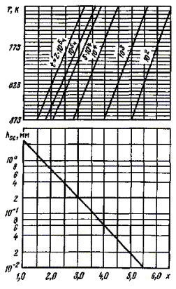
Fig. 5.20.
Diagram of 12Kh18N10T steel carburization in sodium (x = 6050/T –
lgt)
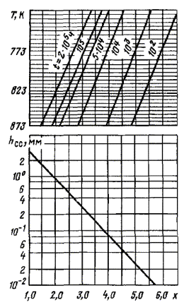
Fig. 5.21.
Diagram of 12Kh16N15M3B steel carburization in sodium (x = 6050/T
– lgt)
5.9.6. The mean
shear stress in keys, dowels, etc., caused by the action of shear forces from
mechanical and compensation loads affecting the equipment, shall not exceed 0.5
[σ], where nominal permissible stress [σ] = RTmt/nmt.
Safety coefficients nmt are assumed in accordance with
Section 3.4 for keys, dowels, etc., and in accordance with Section 3.5
for bolts and pins.
5.9.7. Calculation
for the long-term static strength of sodium-wetted components of the circuit of
austenitic steels if components of carbon or alloyed steels are in the same
circuit, is carried out according to items 5.9.1 - 5.9.3 if the
depth of the carburizing zone hcc for a given time and
temperature does not exceed the design wall thickness of the component.
For the
circuit with reactor-grade sodium, the value of hcc is
determined according to Fig. 5.20 and 5.21.
5.10. CALCULATION FOR PROGRESSIVE FORM CHANGE
5.10.1. The
calculation for progressive form change is carried out in relation to the
components of structure for which residual shape changes during operation are
unacceptable or limited to specified limits according to the normal operation
of the structure (according to the conditions of operability of movable joints,
disassembly of detachable connections, stability of gaps providing hydraulic
characteristics, etc.).
The
recommended method for calculating the progressive form change is given in
Appendix 4.
5.10.2. The
calculation is carried out for normal and abnormal operation, with due regard
to all the design loads specified in item 5.1.3, except for seismic and
vibration ones.
5.10.3. Calculated
values of displacements accumulated in a component of structure during a given
service life, with due regard to the number of repetitions of operating
conditions, shall not exceed the permissible ones established on the grounds of
operational requirements.
5.11. CALCULATION FOR SEISMIC IMPACTS
5.11.1.
General.
5.11.1.1. When
performing calculations for seismic impacts, the following definitions are
additionally used:
Seismic
intensity of the NPI construction site is the intensity of possible seismic
impacts for the construction site with the corresponding categories of
repeatability over a standard period; set in accordance with seismic risk
zoning maps and microzoning of the construction site; measured in magnitude
degrees according to the MSK-64 scale.
Equipment or
pipeline elevation is the height of the anchorage point of the equipment or
pipeline relative to the lower plane of the building foundation.
Safe shutdown
earthquake (SSE) is an earthquake with mean repeatability of up to 10000 years.
Operating
basis earthquake (OBE) is an earthquake with mean repeatability of up to 100
years.
Accelerogram
is the time dependence of the absolute acceleration of the anchorage point of
the equipment or pipeline for one direction for a particular elevation.
Response
spectrum is the set of absolute values of the maximum response accelerations of
a linear-elastic system with one degree of freedom (oscillator) under the
action given by the accelerogram determined depending on the natural frequency
and damping parameter of the oscillator.
Generalized
response spectrum is the spectrum obtained from the results of processing of
response spectra for a set of accelerograms:
(σs)s
– bearing stresses with due regard to seismic loads, MPa (kgf/mm2);
(τs)s
– shear stresses with due regard to seismic loads, MPa (kgf/mm2);
k – relative
damping (in fractions of critical).
5.11.1.2. The
calculation is carried out for an NPI with the site seismic intensity of
magnitude 5 and higher.
The need for
calculations of equipment and pipelines for an NPI with the site seismic
intensity of magnitude 4 is determined by the design (engineering)
organization.
5.11.1.3. These
rules contain the requirements for performing strength calculations at seismic
effects of equipment and pipelines, subdivided into groups A, B and C in
accordance with the NPI Rules.
5.11.1.4. When
calculating, the equipment and pipelines are divided into two categories (I and
II).
5.11.1.5. Category I
includes equipment and pipelines of groups A and B.
5.11.1.6.
Category II includes equipment and pipelines of group C.
5.11.1.7.
Recommended methods for calculating equipment and pipelines for seismic effects
are given in Appendix 9.
5.11.2.
Requirements for calculation.
5.11.2.1. The source
data for the calculation are as follows:
1) effects
from earthquakes (OBE and SSE) in the form of accelerograms and response
spectra for equipment and pipelines for three mutually perpendicular directions
(vertical and two horizontal);
2) loads under
the NO conditions and, if necessary, under the AO and emergency conditions.
5.11.2.2. Seismic
loads on equipment and pipelines are determined with due regard to the
simultaneous seismic effects in two horizontal and one vertical directions.
5.11.2.3. The
following can be used to determine seismic loads:
1) three
accelerograms for three mutually perpendicular directions;
2) reaction
spectra corresponding to given accelerograms;
3) generalized
reaction spectra.
5.11.2.4. Value
of the relative damping is assumed to be equal to k = 0.02. In the
presence of experimental justification the use of other values is allowed.
5.11.2.5. The
strength of equipment and pipelines during seismic impacts is assessed with due
regard to the requirements of item 1.2.14.
5.11.2.6. The
need to take into account combined effects of seismic loads and loads of the AO
and emergency conditions is established by the design engineering organization.
5.11.2.7.
Equipment and pipelines of category I shall be designed on the combination of
loads of NO + SSE and NO + OBE. If the OBE and SSE accelerograms, adopted for
the calculation, differ only in amplitudes, it is allowed not to consider the
combination of NO + OBE loads.
5.11.2.8. Equipment
and pipelines of category II shall be designed on the combination of loads of
NO + OBE.
5.11.2.9. The
calculation is performed using the linear-spectral method (based on response
spectra) or the dynamic analysis method (based on accelerograms).
If the first
eigen frequency of oscillations is more than 20 Hz, the analysis can be
performed with the aid of static methods with multiplication of the
accelerations obtained from the response spectra by the coefficient of 1.3 for
the frequency in the range of 20-33 Hz and the coefficient of 1.0 for the
frequencies above 33 Hz.
5.11.2.10. The
determination of stresses and deformations is allowed under the assumption of a
static impact of loads on equipment and pipelines found by seismic
calculations.
5.11.2.11. Stresses in
the equipment and pipelines shall meet the requirements of Tables 5.14
and 5.15.
5.11.2.12. Mean
bearing stresses shall not exceed the values given in Table 5.16.
5.11.2.13. Mean shear
stresses shall not exceed the values given in Table 5.17.
5.11.2.14. The
cyclic strength is calculated according to Section 5.61
The
calculation is allowed to be carried out using the maximum amplitude of
stresses determined with due regard to the effects of NO + OBE. Provided that,
the number of loading cycles is assumed to be equal to 50.
This
calculation may be omitted if the total damage from loads effecting the
equipment and pipelines, excluding seismic effects during the NPI operation,
does not exceed 0.8.
Table 5.14. Load
combinations and permissible stresses for equipment and pipelines
|
Category
|
Load
combination
|
Design
group of stress categories
|
Permissible
stress
|
|
I
|
NO + SSE
|
(σs)1
|
1.4[σ]
|
|
|
(σs)2
|
1.8[σ]
|
|
NO + OBE
|
(σs)1
|
1.2[σ]
|
|
|
(σs)2
|
1.6[σ]
|
|
II
|
NO + OBE
|
(σs)1
|
1.5[σ]
|
|
|
(σs)2
|
1.9[σ]
|
Note. For the
NPI pipelines which have undergone strength assessment at the stages of static
calculations, it is allowed not to test the strength of seismic loads for
membrane stresses (σs)1.
Table 5.15. Load
combinations and permissible stresses for bolts and pins
|
Categories
|
Load
combination
|
Design
group of stress categories
|
Permissible
stress
|
|
I
|
NO + SSE
|
(σs)mw
|
1.4[σ]w
|
|
|
(σs)4w
|
2.2[σ]w
|
|
NO + OBE
|
(σs)mw
|
1.2[σ]w
|
|
|
(σs)4w
|
2.0[σ]w
|
|
II
|
NO + OBE
|
(σs)mw
|
1.5[σ]w
|
|
|
(σs)4w
|
2.3[σ]w
|
Table 5.16. Load
combinations and permissible bearing stresses
|
Categories
|
Load
combination
|
Stress
category
|
Permissible
stress
|
|
I
|
NO + SSE
|
(σs)s
|
2.7[σ]
|
|
NO + OBE
|
2.5[σ]
|
|
II
|
NO + OBE
|
(σs)s
|
3.0[σ]
|
Table 5.17. Load
combinations and permissible tangential shear stresses
|
Category
|
Load
combination
|
Stress
category
|
Permissible
stresses
|
|
in bolts
and pins
|
in
components of structures other than bolts and pins
|
|
I
|
NO + SSE
|
(τs)s
|
0.7[σ]w
|
0.7[σ]
|
|
NO + OBE
|
0.6[σ]w
|
0.6[σ]
|
|
II
|
NO + OBE
|
(τs)s
|
0.8[σ]w
|
0.8[σ]
|
5.11.2.15. When
calculating the stability, the permissible stresses are assumed to be:
at σkr
<RTp0.2 [σc] =
0.7σkr;
at σkr
≥ RTp0.2 [σс] = 0.7RTp0.2.
5.11.2.1.6.
Assessment of pipelines for permissible stability stresses may be omitted.
5.11.2.17. Permissible
movements (deflection, shift, displacement, etc.) are determined depending on
the operating conditions (selection of clearance, unacceptable skews,
unacceptable collisions, decompression of sealed joints, etc.).
5.11.2.18.
Recommended methods for calculating the seismic effects are given in Appendix 9.
5.12. CALCULATION FOR VIBRATION STRENGTH
5.12.1. The
vibration strength is calculated in relation to the components of structures
subjected to vibration loading.
5.12.2. Calculation
for vibration strength includes:
1)
determination of spectrum of natural oscillation frequencies and check of
condition of their tune-out form determined disturbance frequencies;
2)
verification for the absence of vibro-impact interfaces of components of
structures in order to exclude increased wear;
3) calculation
for cyclic strength with due regard to vibration stresses.
5.12.3. Recommended
methods of calculation and experimental assessment of vibration strength are
given in Appendix 8.
5.12.4. Calculation
for cyclic strength taking into account vibration loading is carried out
according to the methods described in Section 5.6 hereof.
APPENDIX 1
(mandatory)
PHYSICAL AND MECHANICAL PROPERTIES OF STRUCTURAL
MATERIALS
Table P1.1. Mechanical
properties of steels and alloys (both significant figures are included in the
limit)
|
Steel
or alloy grade
|
Products
|
Characteristic
|
Temperature,
K (°C)
|
|
293 (20)
|
323 (50)
|
373 (100)
|
423 (150)
|
473 (200)
|
523 (250)
|
573 (300)
|
623 (350)
|
673 (400)
|
723 (450)
|
773 (500)
|
823 (550)
|
873 (600)
|
|
St3sp5
|
Hot-rolled sectional
shaped and sheet steel up to 20 mm thick
|
RTm, MPa
|
373
|
363
|
353
|
353
|
343
|
323
|
284
|
-
|
-
|
-
|
-
|
-
|
-
|
|
(kgf/mm2)
|
(38)
|
(37)
|
(36)
|
(36)
|
(35)
|
(33)
|
(29)
|
-
|
-
|
-
|
-
|
-
|
-
|
|
RTp0.2, MPa
|
245
|
235
|
235
|
235
|
235
|
206
|
186
|
-
|
-
|
-
|
-
|
-
|
-
|
|
(kgf/mm2)
|
(25)
|
(24)
|
(24)
|
(24)
|
(24)
|
(21)
|
(19)
|
-
|
-
|
-
|
-
|
-
|
-
|
|
A, %
|
26
|
24
|
22
|
20
|
20
|
20
|
20
|
-
|
-
|
-
|
-
|
-
|
-
|
|
Z, %
|
50
|
49
|
49
|
48
|
47
|
47
|
48
|
-
|
-
|
-
|
-
|
-
|
-
|
|
Same, with a thickness
of over 20 to 100 mm
|
RTm, MPa
|
373
|
363
|
353
|
353
|
343
|
323
|
284
|
-
|
-
|
-
|
-
|
-
|
-
|
|
(kgf/mm2)
|
(38)
|
(37)
|
(36)
|
(36)
|
(35)
|
(33)
|
(29)
|
-
|
-
|
-
|
-
|
-
|
-
|
|
RTp0.2, MPa
|
206
|
196
|
196
|
196
|
196
|
177
|
157
|
-
|
-
|
-
|
-
|
-
|
-
|
|
(kgf/mm2)
|
(21)
|
(20)
|
(20)
|
(20)
|
(20)
|
(18)
|
(16)
|
-
|
-
|
-
|
-
|
-
|
-
|
|
A, %
|
23
|
21
|
19
|
18
|
18
|
18
|
18
|
-
|
-
|
-
|
-
|
-
|
-
|
|
Z, %
|
50
|
49
|
49
|
48
|
47
|
47
|
48
|
-
|
-
|
-
|
-
|
-
|
-
|
|
Same, with a thickness
of over 100 mm
|
RTm, MPa
|
373
|
363
|
353
|
353
|
343
|
323
|
284
|
-
|
-
|
-
|
-
|
-
|
-
|
|
(kgf/mm2)
|
(38)
|
(37)
|
(36)
|
(36)
|
(35)
|
(33)
|
(29)
|
-
|
-
|
-
|
-
|
-
|
-
|
|
RTp0.2, MPa
|
206
|
196
|
196
|
196
|
196
|
177
|
157
|
-
|
-
|
-
|
-
|
-
|
-
|
|
(kgf/mm2)
|
(21)
|
(20)
|
(20)
|
(20)
|
(20)
|
(18)
|
(16)
|
-
|
-
|
-
|
-
|
-
|
-
|
|
A, %
|
23
|
21
|
19
|
18
|
18
|
18
|
18
|
-
|
-
|
-
|
-
|
-
|
-
|
|
Z, %
|
50
|
49
|
49
|
48
|
47
|
47
|
48
|
-
|
-
|
-
|
-
|
-
|
-
|
|
Pipes
|
RTm, MPa
|
373
|
363
|
353
|
343
|
343
|
323
|
324
|
-
|
-
|
-
|
-
|
-
|
-
|
|
(kgf/mm2)
|
(38)
|
(37)
|
(36)
|
(35)
|
(35)
|
(33)
|
(33)
|
-
|
-
|
-
|
-
|
-
|
-
|
|
RTp0.2, MPa
|
206
|
196
|
196
|
196
|
196
|
177
|
157
|
-
|
-
|
-
|
-
|
-
|
-
|
|
(kgf/mm2)
|
(21)
|
(20)
|
(20)
|
(20)
|
(20)
|
(18)
|
(16)
|
-
|
-
|
-
|
-
|
-
|
-
|
|
|
A, %
|
23
|
21
|
19
|
18
|
18
|
18
|
18
|
-
|
-
|
-
|
-
|
-
|
-
|
|
|
Z, %
|
50
|
49
|
49
|
48
|
47
|
47
|
48
|
-
|
-
|
-
|
-
|
-
|
-
|
|
|
Forgings with a
diameter or thickness of up to 300 mm, KP175*
|
RTm, MPa
|
355
|
343
|
333
|
333
|
314
|
304
|
275
|
-
|
-
|
-
|
-
|
-
|
-
|
|
|
(kgf/mm2)
|
(36)
|
(35)
|
(34)
|
(34)
|
(32)
|
(31)
|
(28)
|
-
|
-
|
-
|
-
|
-
|
-
|
|
|
RTp0.2, MPa
|
175
|
167
|
167
|
167
|
157
|
147
|
137
|
-
|
-
|
-
|
-
|
-
|
-
|
|
|
(kgf/mm2)
|
(18)
|
(17)
|
(17)
|
(17)
|
(16)
|
(15)
|
(14)
|
-
|
-
|
-
|
-
|
-
|
-
|
|
|
A, %
|
24
|
22
|
20
|
18
|
17
|
17
|
17
|
-
|
-
|
-
|
-
|
-
|
-
|
|
|
Z, %
|
50
|
47
|
44
|
41
|
40
|
40
|
40
|
-
|
-
|
-
|
-
|
-
|
-
|
|
|
Forgings with a
diameter or thickness of up to 300 mm, KP195*
|
RTm, MPa
|
390
|
390
|
373
|
373
|
363
|
333
|
304
|
-
|
-
|
-
|
-
|
-
|
-
|
|
|
(kgf/mm2)
|
(40)
|
(40)
|
(38)
|
(38)
|
(37)
|
(34)
|
(31)
|
-
|
-
|
-
|
-
|
-
|
-
|
|
|
RTp0.2, MPa
|
195
|
195
|
195
|
195
|
177
|
167
|
147
|
-
|
-
|
-
|
-
|
-
|
-
|
|
|
(kgf/mm2)
|
(20)
|
(20)
|
(20)
|
(20)
|
(18)
|
(17)
|
(15)
|
-
|
-
|
-
|
-
|
-
|
-
|
|
|
A, %
|
23
|
21
|
20
|
18
|
18
|
18
|
18
|
-
|
-
|
-
|
-
|
-
|
-
|
|
|
Z, %
|
50
|
47
|
44
|
41
|
40
|
40
|
40
|
-
|
-
|
-
|
-
|
-
|
-
|
|
|
Same, up to 50 mm,
KP215*
|
RTm, MPa
|
420
|
422
|
402
|
402
|
392
|
373
|
333
|
-
|
-
|
-
|
-
|
-
|
-
|
|
|
(kgf/mm2)
|
(44)
|
(43)
|
(41)
|
(41)
|
(40)
|
(38)
|
(34)
|
-
|
-
|
-
|
-
|
-
|
-
|
|
|
RTp0.2, MPa
|
215
|
206
|
206
|
206
|
196
|
196
|
167
|
-
|
-
|
-
|
-
|
-
|
-
|
|
|
(kgf/mm2)
|
(22)
|
(21)
|
(21)
|
(21)
|
(20)
|
(20)
|
(17)
|
-
|
-
|
-
|
-
|
-
|
-
|
|
|
A, %
|
23
|
21
|
20
|
18
|
18
|
18
|
18
|
-
|
-
|
-
|
-
|
-
|
-
|
|
|
Z, %
|
50
|
47
|
44
|
41
|
40
|
40
|
40
|
-
|
-
|
-
|
-
|
-
|
-
|
|
10
|
Cold- and warm-worked
seamless pipes with an outer diameter of 5 to 250 mm, with a wall thickness
of 0.3 to 20 mm, with an outer diameter of 6 to 250 mm, with a wall thickness
of 1.6 to 24 mm; with an outer diameter of 6 to 160 mm, with a wall thickness
of 2 to 22 mm
|
RTm, MPa
|
343
|
333
|
333
|
333
|
333
|
323
|
314
|
294
|
-
|
-
|
-
|
-
|
-
|
|
|
(kgf/mm2)
|
(35)
|
(34)
|
(34)
|
(34)
|
(34)
|
(33)
|
(32)
|
(30)
|
-
|
-
|
-
|
-
|
-
|
|
|
RTp0.2, MPa
|
206
|
196
|
195
|
181
|
176
|
157
|
137
|
118
|
-
|
-
|
-
|
-
|
-
|
|
|
(kgf/mm2)
|
(21)
|
(20)
|
(19)
|
(18.5)
|
(18)
|
(16)
|
(14)
|
(12)
|
-
|
-
|
-
|
-
|
-
|
|
|
A, %
|
24
|
20
|
18
|
18
|
19
|
21
|
23
|
24
|
-
|
-
|
-
|
-
|
-
|
|
|
Z, %
|
50
|
46
|
40
|
40
|
40
|
42
|
44
|
48
|
-
|
-
|
-
|
-
|
-
|
|
|
Sectional hot-rolled
and forged steel with a thickness or diameter of up to 80 mm
|
RTm, MPa
|
333
|
333
|
333
|
333
|
333
|
323
|
314
|
294
|
-
|
-
|
-
|
-
|
-
|
|
|
(kgf/mm2)
|
(34)
|
(34)
|
(34)
|
(34)
|
(34)
|
(33)
|
(32)
|
(30)
|
-
|
-
|
-
|
-
|
-
|
|
|
RTp0.2, MPa
|
186
|
186
|
186
|
177
|
177
|
157
|
137
|
118
|
-
|
-
|
-
|
-
|
-
|
|
|
(kgf/mm2)
|
(09)
|
(19)
|
(19)
|
(18)
|
(18)
|
(16)
|
(14)
|
(12)
|
-
|
-
|
-
|
-
|
-
|
|
|
A, %
|
31
|
28
|
26
|
22
|
25
|
245
|
255
|
28
|
-
|
-
|
-
|
-
|
-
|
|
|
Z, %
|
55
|
50
|
50
|
46
|
44
|
44
|
44
|
46
|
-
|
-
|
-
|
-
|
-
|
|
15
|
Sectional hot-rolled steel
with a thickness or diameter of up to 80 mm
|
RTm, MPa
|
373
|
373
|
363
|
353
|
343
|
333
|
333
|
333
|
-
|
-
|
-
|
-
|
-
|
|
|
(kgf/mm2)
|
(38)
|
(38)
|
(37)
|
(36)
|
(35)
|
(34)
|
(34)
|
(34)
|
-
|
-
|
-
|
-
|
-
|
|
|
RTp0.2, MPa
|
226
|
216
|
216
|
196
|
196
|
196
|
196
|
196
|
-
|
-
|
-
|
-
|
-
|
|
|
(kgf/mm2)
|
(23)
|
(22)
|
(22)
|
(20)
|
(20)
|
(20)
|
(20)
|
(20)
|
-
|
-
|
-
|
-
|
-
|
|
|
A, %
|
27
|
26
|
25
|
25
|
24
|
23
|
23
|
23
|
-
|
-
|
-
|
-
|
-
|
|
|
Z, %
|
55
|
51
|
47
|
43
|
39
|
38
|
38
|
38
|
-
|
-
|
-
|
-
|
-
|
|
|
Forgings with a
diameter of up to 300 mm, KP175*
|
RTm, MPa
|
355
|
343
|
333
|
324
|
314
|
294
|
294
|
294
|
-
|
-
|
-
|
-
|
-
|
|
|
(kgf/mm2)
|
(36)
|
(35)
|
(34)
|
(33)
|
(32)
|
(30)
|
(30)
|
(30)
|
-
|
-
|
-
|
-
|
-
|
|
|
RTp0.2, MPa
|
175
|
167
|
157
|
147
|
147
|
128
|
118
|
118
|
-
|
-
|
-
|
-
|
-
|
|
|
(kgf/mm2)
|
(18)
|
(17)
|
(16)
|
(15)
|
(15)
|
(13)
|
(12)
|
(12)
|
-
|
-
|
-
|
-
|
-
|
|
|
A, %
|
20
|
19
|
18
|
16
|
14
|
14
|
14
|
14
|
-
|
-
|
-
|
-
|
-
|
|
|
Z, %
|
40
|
40
|
40
|
40
|
40
|
40
|
40
|
40
|
-
|
-
|
-
|
-
|
-
|
|
|
Same, up to 100 mm,
KP195*
|
RTm, MPa
|
390
|
383
|
373
|
363
|
353
|
343
|
333
|
324
|
-
|
-
|
-
|
-
|
-
|
|
|
(kgf/mm2)
|
(40)
|
(39)
|
(38)
|
(37)
|
(36)
|
(35)
|
(34)
|
(33)
|
-
|
-
|
-
|
-
|
-
|
|
|
RTp0.2, MPa
|
195
|
195
|
177
|
167
|
167
|
147
|
128
|
128
|
-
|
-
|
-
|
-
|
-
|
|
|
(kgf/mm2)
|
(20)
|
(20)
|
(18)
|
(17)
|
(17)
|
(15)
|
(13)
|
(13)
|
-
|
-
|
-
|
-
|
-
|
|
|
A, %
|
18
|
17
|
16
|
16
|
14
|
14
|
14
|
14
|
-
|
-
|
-
|
-
|
-
|
|
|
Z, %
|
38
|
38
|
38
|
38
|
36
|
36
|
35
|
35
|
-
|
-
|
-
|
-
|
-
|
|
|
Forgings with a
diameter of up to 50 mm, KP215*
|
RTm, MPa
|
430
|
422
|
402
|
392
|
383
|
363
|
363
|
363
|
-
|
-
|
-
|
-
|
-
|
|
|
(kgf/mm2)
|
(44)
|
(43)
|
(41)
|
(40)
|
(3)
|
(37)
|
(37)
|
(37)
|
-
|
-
|
-
|
-
|
-
|
|
|
RTp0.2, MPa
|
215
|
206
|
186
|
177
|
177
|
157
|
147
|
147
|
-
|
-
|
-
|
-
|
-
|
|
|
(kgf/mm2)
|
(22)
|
(21)
|
(19)
|
(18)
|
(18)
|
(16)
|
(15)
|
(15)
|
-
|
-
|
-
|
-
|
-
|
|
|
A, %
|
24
|
21
|
18
|
16
|
14
|
14
|
14
|
14
|
-
|
-
|
-
|
-
|
-
|
|
|
Z, %
|
53
|
47
|
44
|
42
|
40
|
40
|
40
|
40
|
-
|
-
|
-
|
-
|
-
|
|
15L
|
Castings with a wall
thickness of up to 100 mm
|
RTm, MPa
|
392
|
392
|
373
|
363
|
363
|
353
|
343
|
333
|
-
|
-
|
-
|
-
|
-
|
|
|
(kgf/mm2)
|
(40)
|
(40)
|
(38)
|
(37)
|
(37)
|
(36)
|
(35)
|
(34)
|
-
|
-
|
-
|
-
|
-
|
|
|
RTp0.2, MPa
|
196
|
196
|
196
|
177
|
157
|
147
|
138
|
118
|
-
|
-
|
-
|
-
|
-
|
|
|
(kgf/mm2)
|
(20)
|
(20)
|
(20)
|
(18)
|
(16)
|
(15)
|
(14)
|
(12)
|
-
|
-
|
-
|
-
|
-
|
|
|
A, %
|
24
|
23
|
23
|
23
|
22
|
21
|
21
|
21
|
-
|
-
|
-
|
-
|
-
|
|
|
Z, %
|
35
|
35
|
35
|
34
|
34
|
33
|
32
|
30
|
-
|
-
|
-
|
-
|
-
|
|
20
|
Forgings with a
diameter of up to 300 mm, KP175*
|
RTm, MPa
|
355
|
343
|
333
|
323
|
323
|
294
|
294
|
294
|
-
|
-
|
-
|
-
|
-
|
|
|
(kgf/mm2)
|
(36)
|
(35)
|
(34)
|
(33)
|
(33)
|
(30)
|
(30)
|
(30)
|
-
|
-
|
-
|
-
|
-
|
|
|
RTp0.2, MPa
|
175
|
167
|
167
|
167
|
167
|
157
|
147
|
128
|
-
|
-
|
-
|
-
|
-
|
|
|
(kgf/mm2)
|
(18)
|
(17)
|
(17)
|
(17)
|
(17)
|
(16)
|
(15)
|
(13)
|
-
|
-
|
-
|
-
|
-
|
|
|
A, %
|
20
|
20
|
20
|
18
|
17
|
17
|
17
|
17
|
-
|
-
|
-
|
-
|
-
|
|
|
Z, %
|
40
|
40
|
40
|
40
|
40
|
40
|
40
|
40
|
-
|
-
|
-
|
-
|
-
|
|
|
Same, up to 300 mm,
KP195*
|
RTm, MPa
|
390
|
390
|
373
|
363
|
363
|
343
|
333
|
323
|
-
|
-
|
-
|
-
|
-
|
|
|
(kgf/mm2)
|
(40)
|
(40)
|
(38)
|
(37)
|
(37)
|
(35)
|
(34)
|
(33)
|
-
|
-
|
-
|
-
|
-
|
|
|
RTp0.2, MPa
|
195
|
195
|
195
|
195
|
195
|
177
|
157
|
137
|
-
|
-
|
-
|
-
|
-
|
|
|
(kgf/mm2)
|
(20)
|
(20)
|
(20)
|
(20)
|
(20)
|
(18)
|
(16)
|
(14)
|
-
|
-
|
-
|
-
|
-
|
|
|
A, %
|
20
|
20
|
20
|
18
|
17
|
17
|
17
|
17
|
-
|
-
|
-
|
-
|
-
|
|
|
Z, %
|
40
|
40
|
40
|
40
|
40
|
40
|
40
|
40
|
-
|
-
|
-
|
-
|
-
|
|
|
Forgings with a
diameter of up to 300 mm, KP215*
|
RTm, MPa
|
430
|
422
|
422
|
412
|
402
|
402
|
392
|
373
|
-
|
-
|
-
|
-
|
-
|
|
|
(kgf/mm2)
|
(44)
|
(43)
|
(43)
|
(42)
|
(41)
|
(41)
|
(40)
|
(38)
|
-
|
-
|
-
|
-
|
-
|
|
|
RTp0.2, MPa
|
215
|
206
|
206
|
206
|
196
|
196
|
177
|
157
|
-
|
-
|
-
|
-
|
-
|
|
|
(kgf/mm2)
|
(22)
|
(21)
|
(21)
|
(21)
|
(20)
|
(20)
|
(18)
|
(16)
|
-
|
-
|
-
|
-
|
-
|
|
|
A, %
|
20
|
19
|
19
|
18
|
17
|
17
|
17
|
17
|
-
|
-
|
-
|
-
|
-
|
|
|
Z, %
|
40
|
40
|
40
|
40
|
40
|
40
|
40
|
40
|
-
|
-
|
-
|
-
|
-
|
|
|
Same, 100 to 300 mm,
KP245*
|
RTm, MPa
|
470
|
461
|
461
|
451
|
441
|
441
|
432
|
422
|
-
|
-
|
-
|
-
|
-
|
|
|
(kgf/mm2)
|
(48)
|
(47)
|
(47)
|
(46)
|
(45)
|
(45)
|
(44)
|
(43)
|
-
|
-
|
-
|
-
|
-
|
|
|
RTp0.2, MPa
|
245
|
235
|
235
|
235
|
226
|
226
|
196
|
177
|
-
|
-
|
-
|
-
|
-
|
|
|
(kgf/mm2)
|
(25)
|
(24)
|
(24)
|
(24)
|
(23)
|
(23)
|
(20)
|
(18)
|
-
|
-
|
-
|
-
|
-
|
|
|
A, %
|
19
|
18
|
18
|
17
|
16
|
16
|
16
|
16
|
-
|
-
|
-
|
-
|
-
|
|
|
Z, %
|
40
|
40
|
40
|
40
|
40
|
40
|
40
|
40
|
-
|
-
|
-
|
-
|
-
|
|
|
Hot-rolled steel with
a thickness or diameter of up to 80 mm; hot-worked pipes with an outer
diameter of 10 to 465 mm, with a wall thickness of 2 to 60 mm
|
RTm, MPa
|
402
|
392
|
392
|
392
|
373
|
373
|
363
|
353
|
-
|
-
|
-
|
-
|
-
|
|
|
(kgf/mm2)
|
(41)
|
(40)
|
(40)
|
(40)
|
(38)
|
(38)
|
(37)
|
(36)
|
-
|
-
|
-
|
-
|
-
|
|
|
RTp0.2, MPa
|
216
|
206
|
206
|
206
|
196
|
196
|
177
|
157
|
-
|
-
|
-
|
-
|
-
|
|
|
(kgf/mm2)
|
(22)
|
(21)
|
(21)
|
(21)
|
(20)
|
(20)
|
(18)
|
(16)
|
-
|
-
|
-
|
-
|
-
|
|
|
A, %
|
21
|
20
|
19
|
18
|
17
|
17
|
17
|
17
|
-
|
-
|
-
|
-
|
-
|
|
|
Z, %
|
40
|
40
|
38
|
38
|
38
|
38
|
40
|
42
|
-
|
-
|
-
|
-
|
-
|
|
|
Annealed, high-temper
sheets with a thickness of 4 to 80 mm
|
RTm, MPa
|
373
|
363
|
353
|
343
|
343
|
333
|
333
|
323
|
-
|
-
|
-
|
-
|
-
|
|
|
(kgf/mm2)
|
(3)
|
(37)
|
(36)
|
(35)
|
(35)
|
(34)
|
(34)
|
(33)
|
-
|
-
|
-
|
-
|
-
|
|
|
RTp0.2, MPa
|
216
|
216
|
216
|
206
|
206
|
196
|
176
|
157
|
-
|
-
|
-
|
-
|
-
|
|
|
(kgf/mm2)
|
(22)
|
(22)
|
(22)
|
(21)
|
(21)
|
(20)
|
(18)
|
(16)
|
-
|
-
|
-
|
-
|
-
|
|
|
A, %
|
28
|
27
|
27
|
25
|
24
|
24
|
24
|
24
|
-
|
-
|
-
|
-
|
-
|
|
|
Z, %
|
45
|
43
|
43
|
42
|
42
|
42
|
44
|
46
|
-
|
-
|
-
|
-
|
-
|
|
|
Parent sheets with a
thickness of 20 to 250 mm (transverse direction)
|
RTm, MPa
|
353
|
343
|
334
|
324
|
304
|
294
|
284
|
275
|
-
|
-
|
-
|
-
|
-
|
|
|
(kgf/mm2)
|
(36)
|
(35)
|
(34)
|
(33)
|
(31)
|
(30)
|
(29)
|
(28)
|
-
|
-
|
-
|
-
|
-
|
|
|
RTp0.2, MPa
|
176
|
176
|
176
|
157
|
157
|
147
|
147
|
137
|
-
|
-
|
-
|
-
|
-
|
|
|
(kgf/mm2)
|
(18)
|
(18)
|
(18)
|
(16)
|
(16)
|
(15)
|
(15)
|
(14)
|
-
|
-
|
-
|
-
|
-
|
|
|
A, %
|
20
|
20
|
20
|
19
|
19
|
19
|
18
|
18
|
-
|
-
|
-
|
-
|
-
|
|
|
Z, %
|
45
|
45
|
45
|
45
|
45
|
45
|
45
|
45
|
-
|
-
|
-
|
-
|
-
|
|
20L
|
Castings with a wall
thickness of up to 100 mm
|
RTm, MPa
|
412
|
412
|
412
|
392
|
370
|
370
|
370
|
360
|
-
|
-
|
-
|
-
|
-
|
|
|
(kgf/mm2)
|
(42)
|
(42)
|
(42)
|
(40)
|
(38)
|
(38)
|
(38)
|
(37)
|
-
|
-
|
-
|
-
|
-
|
|
|
RTp0.2, MPa
|
216
|
216
|
196
|
176
|
170
|
165
|
157
|
137
|
-
|
-
|
-
|
-
|
-
|
|
|
(kgf/mm2)
|
(22)
|
(22)
|
(20)
|
(18)
|
(17.5)
|
(17)
|
(16)
|
(14)
|
-
|
-
|
-
|
-
|
-
|
|
|
A, %
|
22
|
21
|
20
|
19
|
18
|
18
|
18
|
18
|
-
|
-
|
-
|
-
|
-
|
|
|
Z, %
|
35
|
35
|
35
|
35
|
35
|
34
|
33
|
32
|
-
|
-
|
-
|
-
|
-
|
|
20K
|
Sheets with a
thickness of 4 to 60 mm
|
RTm, MPa
|
402
|
397
|
397
|
392
|
392
|
392
|
373
|
363
|
-
|
-
|
-
|
-
|
-
|
|
|
(kgf/mm2)
|
(41)
|
(40.5)
|
(40.5)
|
(40)
|
(40)
|
(40)
|
(38)
|
(37)
|
-
|
-
|
-
|
-
|
-
|
|
|
RTp0.2, MPa
|
216
|
206
|
206
|
206
|
196
|
196
|
177
|
157
|
-
|
-
|
-
|
-
|
-
|
|
|
(kgf/mm2)
|
(22)
|
(21)
|
(21)
|
(21)
|
(20)
|
(20)
|
(18)
|
(16)
|
-
|
-
|
-
|
-
|
-
|
|
|
A, %
|
23
|
21
|
20
|
20
|
19
|
19
|
19
|
19
|
-
|
-
|
-
|
-
|
-
|
|
|
Z, %
|
50
|
48
|
47
|
47
|
47
|
47
|
49
|
51
|
-
|
-
|
-
|
-
|
-
|
|
22К
|
Sheets with a
thickness of 70 to 170 mm, KP215*
|
RTm, MPa
|
430
|
430
|
430
|
430
|
430
|
421
|
412
|
392
|
-
|
-
|
-
|
-
|
-
|
|
|
(kgf/mm2)
|
(44)
|
(44)
|
(44)
|
(44)
|
(44)
|
(43)
|
(42)
|
(40)
|
-
|
-
|
-
|
-
|
-
|
|
|
RTp0.2, MPa
|
215
|
206
|
196
|
186
|
186
|
186
|
186
|
177
|
-
|
-
|
-
|
-
|
-
|
|
|
(kgf/mm2)
|
(22)
|
(21)
|
(20)
|
(19)
|
(19)
|
(19)
|
(19)
|
(18)
|
-
|
-
|
-
|
-
|
-
|
|
|
A, %
|
18
|
18
|
18
|
17
|
17
|
16
|
17
|
18
|
-
|
-
|
-
|
-
|
-
|
|
|
Z, %
|
40
|
40
|
39
|
38
|
38
|
38
|
39
|
40
|
-
|
-
|
-
|
-
|
-
|
|
|
Forgings with a
diameter of 300 to 800 mm, KP195*
|
RTm, MPa
|
390
|
390
|
390
|
383
|
373
|
363
|
353
|
353
|
-
|
-
|
-
|
-
|
-
|
|
|
(kgf/mm2)
|
(40)
|
(40)
|
(40)
|
(39)
|
(38)
|
(37)
|
(36)
|
(36)
|
-
|
-
|
-
|
-
|
-
|
|
|
RTp0.2, MPa
|
195
|
186
|
177
|
167
|
167
|
157
|
157
|
137
|
-
|
-
|
-
|
-
|
-
|
|
|
(kgf/mm2)
|
(20)
|
(19)
|
(18)
|
(17)
|
(17)
|
(16)
|
(16)
|
(14)
|
-
|
-
|
-
|
-
|
-
|
|
|
A, %
|
18
|
15
|
13
|
13
|
13
|
13
|
13
|
13
|
-
|
-
|
-
|
-
|
-
|
|
|
Z, %
|
38
|
38
|
38
|
36
|
36
|
35
|
34
|
34
|
-
|
-
|
-
|
-
|
-
|
|
|
Same, 100 to 800 mm,
KP215*
|
RTm, MPa
|
430
|
392
|
392
|
392
|
392
|
392
|
353
|
343
|
-
|
-
|
-
|
-
|
-
|
|
|
(kgf/mm2)
|
(44)
|
(40)
|
(40)
|
(40)
|
(40)
|
(40)
|
(36)
|
(35)
|
-
|
-
|
-
|
-
|
-
|
|
|
RTp0.2, MPa
|
215
|
206
|
196
|
186
|
186
|
186
|
186
|
177
|
-
|
-
|
-
|
-
|
-
|
|
|
(kgf/mm2)
|
(22)
|
(21)
|
(20)
|
(19)
|
(19)
|
(19)
|
(19)
|
(18)
|
-
|
-
|
-
|
-
|
-
|
|
|
A, %
|
16
|
14
|
11
|
11
|
11
|
11
|
11
|
11
|
-
|
-
|
-
|
-
|
-
|
|
|
Z, %
|
35
|
35
|
35
|
33
|
33
|
32
|
31
|
31
|
-
|
-
|
-
|
-
|
-
|
|
25
|
Forgings with a
diameter of up to 500 mm, KP175*
|
RTm, MPa
|
350
|
343
|
333
|
323
|
323
|
304
|
294
|
294
|
-
|
-
|
-
|
-
|
-
|
|
|
(kgf/mm2)
|
(36)
|
(35)
|
(34)
|
(33)
|
(33)
|
(31)
|
(30)
|
(30)
|
-
|
-
|
-
|
-
|
-
|
|
|
RTp0.2, MPa
|
175
|
167
|
157
|
147
|
137
|
128
|
118
|
108
|
-
|
-
|
-
|
-
|
-
|
|
|
(kgf/mm2)
|
(18)
|
(17)
|
(16)
|
(15)
|
(14)
|
(13)
|
(12)
|
(11)
|
-
|
-
|
-
|
-
|
-
|
|
|
A, %
|
22
|
22
|
22
|
22
|
22
|
22
|
22
|
22
|
-
|
-
|
-
|
-
|
-
|
|
|
Z, %
|
45
|
45
|
45
|
45
|
45
|
45
|
45
|
45
|
-
|
-
|
-
|
-
|
-
|
|
|
Same, up to 500 mm,
KP195*
|
RTm, MPa
|
390
|
390
|
373
|
363
|
363
|
343
|
333
|
323
|
-
|
-
|
-
|
-
|
-
|
|
|
(kgf/mm2)
|
(40)
|
(40)
|
(38)
|
(37)
|
(37)
|
(35)
|
(34)
|
(33)
|
-
|
-
|
-
|
-
|
-
|
|
|
RTp0.2, MPa
|
195
|
195
|
177
|
167
|
157
|
137
|
128
|
118
|
-
|
-
|
-
|
-
|
-
|
|
|
(kgf/mm2)
|
(20)
|
(20)
|
(18)
|
(17)
|
(16)
|
(14)
|
(13)
|
(12)
|
-
|
-
|
-
|
-
|
-
|
|
|
A, %
|
20
|
20
|
20
|
20
|
20
|
20
|
20
|
20
|
-
|
-
|
-
|
-
|
-
|
|
|
Z, %
|
45
|
45
|
45
|
45
|
45
|
45
|
45
|
44
|
-
|
-
|
-
|
-
|
-
|
|
|
Same, up to 300 mm,
KP215*
|
RTm, MPa
|
430
|
422
|
422
|
412
|
402
|
402
|
402
|
373
|
-
|
-
|
-
|
-
|
-
|
|
|
(kgf/mm2)
|
(44)
|
(43)
|
(43)
|
(42)
|
(41)
|
(41)
|
(41)
|
(38)
|
-
|
-
|
-
|
-
|
-
|
|
|
RTp0.2, MPa
|
215
|
206
|
196
|
177
|
167
|
147
|
137
|
118
|
-
|
-
|
-
|
-
|
-
|
|
|
(kgf/mm2)
|
(22)
|
(21)
|
(20)
|
(18)
|
(17)
|
(15)
|
(14)
|
(12)
|
-
|
-
|
-
|
-
|
-
|
|
|
A, %
|
20
|
20
|
20
|
19
|
19
|
19
|
19
|
19
|
-
|
-
|
-
|
-
|
-
|
|
|
Z, %
|
45
|
45
|
45
|
45
|
45
|
45
|
45
|
44
|
-
|
-
|
-
|
-
|
-
|
|
|
Same, up to 100 mm,
KP245*
|
RTm, MPa
|
470
|
461
|
461
|
451
|
441
|
441
|
441
|
412
|
-
|
-
|
-
|
-
|
-
|
|
|
(kgf/mm2)
|
(48)
|
(47)
|
(47)
|
(46)
|
(45)
|
(45)
|
(45)
|
(42)
|
-
|
-
|
-
|
-
|
-
|
|
|
RTp0.2, MPa
|
245
|
235
|
226
|
206
|
196
|
167
|
157
|
118
|
-
|
-
|
-
|
-
|
-
|
|
|
(kgf/mm2)
|
(25)
|
(24)
|
(23)
|
(21)
|
(20)
|
(17)
|
(16)
|
(12)
|
-
|
-
|
-
|
-
|
-
|
|
|
A, %
|
20
|
20
|
20
|
19
|
19
|
19
|
19
|
19
|
-
|
-
|
-
|
-
|
-
|
|
|
Z, %
|
45
|
45
|
45
|
45
|
45
|
45
|
45
|
44
|
-
|
-
|
-
|
-
|
-
|
|
|
Forgings with a
diameter of 100 to 300 mm, KP275*
|
RTm, MPa
|
530
|
510
|
500
|
481
|
481
|
451
|
441
|
441
|
-
|
-
|
-
|
-
|
-
|
|
|
(kgf/mm2)
|
(54)
|
(52)
|
(51)
|
(49)
|
(49)
|
(46)
|
(45)
|
(445)
|
-
|
-
|
-
|
-
|
-
|
|
|
RTp0.2, MPa
|
275
|
255
|
245
|
226
|
216
|
196
|
186
|
167
|
-
|
-
|
-
|
-
|
-
|
|
|
(kgf/mm2)
|
(28)
|
(26)
|
(25)
|
(23)
|
(22)
|
(20)
|
(19)
|
(17)
|
-
|
-
|
-
|
-
|
-
|
|
|
A, %
|
17
|
17
|
17
|
17
|
17
|
17
|
17
|
17
|
-
|
-
|
-
|
-
|
-
|
|
|
Z, %
|
38
|
38
|
38
|
38
|
38
|
38
|
38
|
38
|
-
|
-
|
-
|
-
|
-
|
|
25L
|
Castings with a wall
thickness of up to 100 mm
|
RTm, MPa
|
441
|
432
|
432
|
422
|
422
|
400
|
380
|
370
|
-
|
-
|
-
|
-
|
-
|
|
|
(kgf/mm2)
|
(45)
|
(44)
|
(44)
|
(43)
|
(43)
|
(41)
|
(39)
|
(38)
|
-
|
-
|
-
|
-
|
-
|
|
|
RTp0.2, MPa
|
235
|
226
|
216
|
196
|
180
|
175
|
170
|
150
|
-
|
-
|
-
|
-
|
-
|
|
|
(kgf/mm2)
|
(24)
|
(23)
|
(22)
|
(20)
|
(18.5)
|
(18)
|
(17.5)
|
(15.5)
|
-
|
-
|
-
|
-
|
-
|
|
|
A, %
|
19
|
18
|
17
|
17
|
16
|
16
|
16
|
16
|
-
|
-
|
-
|
-
|
-
|
|
|
Z, %
|
30
|
30
|
30
|
30
|
30
|
30
|
28
|
26
|
-
|
-
|
-
|
-
|
-
|
|
30
|
Forgings with a
diameter of 300 to 800 mm, KP175*
|
RTm, MPa
|
355
|
355
|
343
|
343
|
343
|
333
|
333
|
333
|
-
|
-
|
-
|
-
|
-
|
|
|
(kgf/mm2)
|
(36)
|
(36)
|
(35)
|
(35)
|
(35)
|
(34)
|
(34)
|
(34)
|
-
|
-
|
-
|
-
|
-
|
|
|
RTp0.2, MPa
|
175
|
175
|
175
|
175
|
167
|
137
|
108
|
98
|
-
|
-
|
-
|
-
|
-
|
|
|
(kgf/mm2)
|
(18)
|
(18)
|
(18)
|
(18)
|
(17)
|
(14)
|
(11)
|
(10)
|
-
|
-
|
-
|
-
|
-
|
|
|
A, %
|
20
|
20
|
18
|
17
|
16
|
16
|
16
|
16
|
-
|
-
|
-
|
-
|
-
|
|
|
Z, %
|
40
|
40
|
40
|
40
|
40
|
40
|
40
|
40
|
-
|
-
|
-
|
-
|
-
|
|
|
Same, 100 to 800 mm,
KP195*
|
RTm, MPa
|
390
|
390
|
390
|
373
|
373
|
373
|
373
|
373
|
-
|
-
|
-
|
-
|
-
|
|
|
(kgf/mm2)
|
(40)
|
(40)
|
(40)
|
(38)
|
(38)
|
(38)
|
(38)
|
(38)
|
-
|
-
|
-
|
-
|
-
|
|
|
RTp0.2, MPa
|
195
|
195
|
195
|
195
|
195
|
147
|
118
|
108
|
-
|
-
|
-
|
-
|
-
|
|
|
(kgf/mm2)
|
(20)
|
(20)
|
(20)
|
(20)
|
(20)
|
(15)
|
(12)
|
(11)
|
-
|
-
|
-
|
-
|
-
|
|
|
A, %
|
18
|
17
|
16
|
15
|
14
|
14
|
14
|
14
|
-
|
-
|
-
|
-
|
-
|
|
|
Z, %
|
38
|
38
|
38
|
38
|
38
|
38
|
37
|
37
|
-
|
-
|
-
|
-
|
-
|
|
|
Forgings with a
diameter of over 100 to 800 mm, KP215*
|
RTm, MPa
|
430
|
430
|
422
|
412
|
412
|
402
|
402
|
402
|
-
|
-
|
-
|
-
|
-
|
|
|
(kgf/mm2)
|
(44)
|
(44)
|
(43)
|
(42)
|
(42)
|
(41)
|
(41)
|
(41)
|
-
|
-
|
-
|
-
|
-
|
|
|
RTp0.2, MPa
|
215
|
215
|
215
|
215
|
206
|
167
|
128
|
118
|
-
|
-
|
-
|
-
|
-
|
|
|
(kgf/mm2)
|
(22)
|
(22)
|
(22)
|
(22)
|
(21)
|
(17)
|
(13)
|
(12)
|
-
|
-
|
-
|
-
|
-
|
|
|
A, %
|
16
|
15
|
14
|
14
|
13
|
13
|
13
|
13
|
-
|
-
|
-
|
-
|
-
|
|
|
Z, %
|
35
|
35
|
35
|
35
|
35
|
35
|
34
|
34
|
-
|
-
|
-
|
-
|
-
|
|
|
Same, up to 500 mm,
KP245*
|
RTm, MPa
|
470
|
470
|
461
|
451
|
441
|
441
|
441
|
441
|
-
|
-
|
-
|
-
|
-
|
|
|
(kgf/mm2)
|
(48)
|
(48)
|
(47)
|
(46)
|
(45)
|
(45)
|
(45)
|
(45)
|
-
|
-
|
-
|
-
|
-
|
|
|
RTp0.2, MPa
|
245
|
245
|
245
|
245
|
235
|
196
|
147
|
137
|
-
|
-
|
-
|
-
|
-
|
|
|
(kgf/mm2)
|
(25)
|
(25)
|
(25)
|
(25)
|
(24)
|
(20)
|
(15)
|
(14)
|
-
|
-
|
-
|
-
|
-
|
|
|
A, %
|
16
|
15
|
14
|
14
|
13
|
13
|
13
|
13
|
-
|
-
|
-
|
-
|
-
|
|
|
Z, %
|
35
|
35
|
35
|
35
|
35
|
35
|
34
|
34
|
-
|
-
|
-
|
-
|
-
|
|
35
|
Sectional hot-rolled
steel with a diameter or thickness of up to 80 mm
|
RTm, MPa
|
530
|
530
|
520
|
510
|
510
|
500
|
500
|
500
|
-
|
-
|
-
|
-
|
-
|
|
|
(kgf/mm2)
|
(54)
|
(54)
|
(53)
|
(52)
|
(52)
|
(51)
|
(51)
|
(51)
|
-
|
-
|
-
|
-
|
-
|
|
|
RTp0.2, MPa
|
314
|
304
|
294
|
294
|
294
|
245
|
196
|
177
|
-
|
-
|
-
|
-
|
-
|
|
|
(kgf/mm2)
|
(32)
|
(31)
|
(30)
|
(30)
|
(30)
|
(25)
|
(20)
|
(18)
|
-
|
-
|
-
|
-
|
-
|
|
|
A, %
|
20
|
17
|
13
|
10
|
7
|
12
|
17
|
18
|
-
|
-
|
-
|
-
|
-
|
|
|
Z, %
|
45
|
45
|
45
|
45
|
45
|
45
|
45
|
45
|
-
|
-
|
-
|
-
|
-
|
|
|
Forgings with a diameter
of 500 to 800 mm, KP175*
|
RTm, MPa
|
355
|
355
|
343
|
343
|
343
|
333
|
333
|
333
|
-
|
-
|
-
|
-
|
-
|
|
|
(kgf/mm2)
|
(36)
|
(36)
|
(35)
|
(35)
|
(35)
|
(34)
|
(34)
|
(34)
|
-
|
-
|
-
|
-
|
-
|
|
|
RTp0.2, MPa
|
175
|
167
|
167
|
167
|
167
|
137
|
108
|
98
|
-
|
-
|
-
|
-
|
-
|
|
|
(kgf/mm2)
|
(18)
|
(17)
|
(17)
|
(17)
|
(17)
|
(14)
|
(11)
|
(10)
|
-
|
-
|
-
|
-
|
-
|
|
|
A, %
|
20
|
17
|
13
|
10
|
7
|
12
|
17
|
18
|
-
|
-
|
-
|
-
|
-
|
|
|
Z, %
|
40
|
40
|
40
|
40
|
40
|
40
|
40
|
40
|
-
|
-
|
-
|
-
|
-
|
|
|
Forgings with a
diameter of 300 to 800 mm, KP195*
|
RTm, MPa
|
390
|
390
|
390
|
373
|
373
|
373
|
373
|
373
|
-
|
-
|
-
|
-
|
-
|
|
|
(kgf/mm2)
|
(40)
|
(40)
|
(40)
|
(38)
|
(38)
|
(38)
|
(38)
|
(38)
|
-
|
-
|
-
|
-
|
-
|
|
|
RTp0.2, MPa
|
195
|
195
|
195
|
195
|
195
|
157
|
128
|
108
|
-
|
-
|
-
|
-
|
-
|
|
|
(kgf/mm2)
|
(20)
|
(20)
|
(20)
|
(20)
|
(20)
|
(16)
|
(13)
|
(11)
|
-
|
-
|
-
|
-
|
-
|
|
|
A, %
|
17
|
15
|
12
|
9
|
6
|
10
|
14
|
16
|
-
|
-
|
-
|
-
|
-
|
|
|
Z, %
|
135
|
35
|
35
|
35
|
35
|
35
|
35
|
35
|
-
|
-
|
-
|
-
|
-
|
|
|
Same, 100 to 800 mm,
KP215*
|
RTm, MPa
|
430
|
430
|
422
|
412
|
412
|
402
|
402
|
402
|
-
|
-
|
-
|
-
|
-
|
|
|
(kgf/mm2)
|
(44)
|
(44)
|
(43)
|
(42)
|
(42)
|
(41)
|
(41)
|
(41)
|
-
|
-
|
-
|
-
|
-
|
|
|
RTp0.2, MPa
|
215
|
206
|
206
|
206
|
206
|
177
|
437
|
128
|
-
|
-
|
-
|
-
|
-
|
|
|
(kgf/mm2)
|
(22)
|
(21)
|
(21)
|
(21)
|
(21)
|
(18)
|
(14)
|
(13)
|
-
|
-
|
-
|
-
|
-
|
|
|
A, %
|
15
|
12
|
9
|
6
|
5
|
9
|
13
|
14
|
-
|
-
|
-
|
-
|
-
|
|
|
Z, %
|
32
|
32
|
32
|
32
|
32
|
32
|
32
|
32
|
-
|
-
|
-
|
-
|
-
|
|
|
Same, up to 500 mm,
KP245*
|
RTm, MPa
|
470
|
461
|
451
|
441
|
441
|
441
|
441
|
441
|
-
|
-
|
-
|
-
|
-
|
|
|
(kgf/mm2)
|
(48)
|
(47)
|
(46)
|
(45)
|
(45)
|
(45)
|
(45)
|
(45)
|
-
|
-
|
-
|
-
|
-
|
|
|
RTp0.2, MPa
|
245
|
235
|
226
|
226
|
226
|
177
|
157
|
137
|
-
|
-
|
-
|
-
|
-
|
|
|
(kgf/mm2)
|
(25)
|
(24)
|
(23)
|
(23)
|
(23)
|
(18)
|
(16)
|
(14)
|
-
|
-
|
-
|
-
|
-
|
|
|
A, %
|
17
|
15
|
12
|
9
|
6
|
10
|
14
|
16
|
-
|
-
|
-
|
-
|
-
|
|
|
Z, %
|
35
|
35
|
35
|
35
|
35
|
35
|
35
|
35
|
-
|
-
|
-
|
-
|
-
|
|
|
Same, up to 300 mm,
KP275*
|
RTm, MPa
|
530
|
530
|
530
|
530
|
530
|
519
|
510
|
441
|
-
|
-
|
-
|
-
|
-
|
|
|
(kgf/mm2)
|
(54)
|
(54)
|
(54)
|
(54)
|
(54)
|
(53)
|
(52)
|
(45)
|
-
|
-
|
-
|
-
|
-
|
|
|
RTp0.2, MPa
|
275
|
265
|
265
|
265
|
245
|
225
|
216
|
196
|
-
|
-
|
-
|
-
|
-
|
|
|
(kgf/mm2)
|
(28)
|
(27)
|
(27)
|
(27)
|
(25)
|
(23)
|
(22)
|
(20)
|
-
|
-
|
-
|
-
|
-
|
|
|
A, %
|
17
|
15
|
12
|
9
|
6
|
10
|
14
|
16
|
-
|
-
|
-
|
-
|
-
|
|
|
Z, %
|
38
|
38
|
38
|
38
|
38
|
38
|
38
|
38
|
-
|
-
|
-
|
-
|
-
|
|
|
Forgings with a
diameter of up to 100 mm, KP315*
|
RTm, MPa
|
570
|
570
|
559
|
549
|
540
|
540
|
540
|
540
|
-
|
-
|
-
|
-
|
-
|
|
|
(kgf/mm2)
|
(58)
|
(58)
|
(57)
|
(56)
|
(55)
|
(55)
|
(55)
|
(55)
|
-
|
-
|
-
|
-
|
-
|
|
|
RTp0.2, MPa
|
315
|
304
|
304
|
294
|
274
|
255
|
245
|
225
|
-
|
-
|
-
|
-
|
-
|
|
|
(kgf/mm2)
|
(32)
|
(31)
|
(31)
|
(30)
|
(28)
|
(26)
|
(25)
|
(23)
|
-
|
-
|
-
|
-
|
-
|
|
|
A, %
|
15
|
13
|
11
|
9
|
6
|
8
|
11
|
12
|
-
|
-
|
-
|
-
|
-
|
|
|
Z, %
|
35
|
35
|
34
|
34
|
34
|
34
|
35
|
-35
|
-
|
-
|
-
|
-
|
-
|
|
|
Fastener blanks with a
diameter of up to 300 mm, KP275*
|
RTm, MPa
|
530
|
530
|
530
|
520
|
510
|
500
|
500
|
500
|
-
|
-
|
-
|
-
|
-
|
|
|
(kgf/mm2)
|
(54)
|
(54)
|
(54)
|
(53)
|
(52)
|
(51)
|
(51)
|
(51)
|
-
|
-
|
-
|
-
|
-
|
|
|
RTp0.2, MPa
|
275
|
255
|
235
|
225
|
225
|
186
|
147
|
127
|
-
|
-
|
-
|
-
|
-
|
|
|
(kgf/mm2)
|
(28)
|
(26)
|
(24)
|
(23)
|
(23)
|
(19)
|
(15)
|
(13)
|
-
|
-
|
-
|
-
|
-
|
|
|
A, %
|
17
|
14
|
10
|
7
|
5
|
8
|
14
|
15
|
-
|
-
|
-
|
-
|
-
|
|
|
Z, %
|
38
|
38
|
38
|
38
|
38
|
38
|
38
|
38
|
-
|
-
|
-
|
-
|
-
|
|
40
|
Forgings with a
diameter of 300 to 800 mm, KP215*
|
RTm, MPa
|
430
|
412
|
412
|
402
|
402
|
402
|
392
|
373
|
-
|
-
|
-
|
-
|
-
|
|
|
(kgf/mm2)
|
(44)
|
(42)
|
(42)
|
(41)
|
(41)
|
(41)
|
(40)
|
(38)
|
-
|
-
|
-
|
-
|
-
|
|
|
RTp0.2, MPa
|
215
|
196
|
186
|
177
|
157
|
57
|
157
|
147
|
-
|
-
|
-
|
-
|
-
|
|
|
(kgf/mm2)
|
(22)
|
(20)
|
(19)
|
(18)
|
(16)
|
(16)
|
(16)
|
(15)
|
-
|
-
|
-
|
-
|
-
|
|
|
A, %
|
16
|
15
|
15
|
13
|
13
|
13
|
13
|
13
|
-
|
-
|
-
|
-
|
-
|
|
|
Z, %
|
35
|
35
|
35
|
35
|
35
|
34
|
33
|
33
|
-
|
-
|
-
|
-
|
-
|
|
|
Forgings with a
diameter of 100 to 500 mm, KP245*
|
RTm, MPa
|
470
|
451
|
451
|
441
|
422
|
422
|
422
|
412
|
-
|
-
|
-
|
-
|
-
|
|
|
(kgf/mm2)
|
(48)
|
(46)
|
(46)
|
(45)
|
(43)
|
(43)
|
(43)
|
(42)
|
-
|
-
|
-
|
-
|
-
|
|
|
RTp0.2, MPa
|
245
|
226
|
206
|
196
|
196
|
177
|
177
|
167
|
-
|
-
|
-
|
-
|
-
|
|
|
(kgf/mm2)
|
(25)
|
(23)
|
(21)
|
(20)
|
(20)
|
(18)
|
(18)
|
(17)
|
-
|
-
|
-
|
-
|
-
|
|
|
A, %
|
16
|
15
|
15
|
13
|
13
|
13
|
13
|
13
|
-
|
-
|
-
|
-
|
-
|
|
|
Z, %
|
35
|
35
|
35
|
35
|
35
|
34
|
33
|
33
|
-
|
-
|
-
|
-
|
-
|
|
|
Same, up to 800 mm,
KP275*
|
RTm, MPa
|
530
|
510
|
500
|
491
|
491
|
491
|
471
|
461
|
-
|
-
|
-
|
-
|
-
|
|
|
(kgf/mm2)
|
(54)
|
(52)
|
(51)
|
(50)
|
(50)
|
(50)
|
(48)
|
(47)
|
-
|
-
|
-
|
-
|
-
|
|
|
RTp0.2, MPa
|
275
|
255
|
235
|
216
|
206
|
196
|
196
|
196
|
-
|
-
|
-
|
-
|
-
|
|
|
(kgf/mm2)
|
(28)
|
(26)
|
(24)
|
(22)
|
(21)
|
(20)
|
(20)
|
(20)
|
-
|
-
|
-
|
-
|
-
|
|
|
A, %
|
13
|
12
|
11
|
11
|
11
|
11
|
11
|
11
|
-
|
-
|
-
|
-
|
-
|
|
|
Z, %
|
30
|
30
|
30
|
30
|
30
|
29
|
28
|
28
|
-
|
-
|
-
|
-
|
-
|
|
|
Same, 100 to 300 mm,
KP315*
|
RTm, MPa
|
570
|
549
|
540
|
530
|
510
|
510
|
510
|
491
|
-
|
-
|
-
|
-
|
-
|
|
|
(kgf/mm2)
|
(58)
|
(56)
|
(55)
|
(54)
|
(52)
|
(52)
|
(52)
|
(50)
|
-
|
-
|
-
|
-
|
-
|
|
|
RTp0.2, MPa
|
315
|
294
|
255
|
245
|
235
|
226
|
226
|
216
|
-
|
-
|
-
|
-
|
-
|
|
|
(kgf/mm2)
|
(32)
|
(30)
|
(26)
|
(25)
|
(24)
|
(23)
|
(23)
|
(22)
|
-
|
-
|
-
|
-
|
-
|
|
|
A, %
|
13
|
12
|
11
|
12
|
12
|
12
|
12
|
12
|
-
|
-
|
-
|
-
|
-
|
|
|
Z, %
|
30
|
30
|
30
|
30
|
30
|
29
|
28
|
28
|
-
|
-
|
-
|
-
|
-
|
|
|
Same, up to 100 mm,
KP345*
|
RTm, MPa
|
590
|
569
|
559
|
549
|
530
|
530
|
530
|
510
|
-
|
-
|
-
|
-
|
-
|
|
|
(kgf/mm2)
|
(60)
|
(58)
|
(57)
|
(56)
|
(54)
|
(54)
|
(54)
|
(52)
|
-
|
-
|
-
|
-
|
-
|
|
|
RTp0.2, MPa
|
345
|
312
|
294
|
275
|
255
|
245
|
245
|
235
|
-
|
-
|
-
|
-
|
-
|
|
|
(kgf/mm2)
|
(35)
|
(32)
|
(30)
|
(28)
|
(26)
|
(25)
|
(25)
|
(24)
|
-
|
-
|
-
|
-
|
-
|
|
|
A, %
|
18
|
17
|
16
|
15
|
14
|
14
|
14
|
14
|
-
|
-
|
-
|
-
|
-
|
|
|
Z, %
|
45
|
45
|
45
|
45
|
45
|
45
|
45
|
45
|
-
|
-
|
-
|
-
|
-
|
|
|
Fastener blanks with a
diameter of up to 300 mm, KP295*
|
RTm, MPa
|
549
|
520
|
520
|
510
|
510
|
510
|
500
|
471
|
-
|
-
|
-
|
-
|
-
|
|
|
(kgf/mm2)
|
(56)
|
(53)
|
(53)
|
(52)
|
(52)
|
(52)
|
(51)
|
(48)
|
-
|
-
|
-
|
-
|
-
|
|
|
RTp0.2, MPa
|
295
|
265
|
255
|
235
|
216
|
216
|
216
|
196
|
-
|
-
|
-
|
-
|
-
|
|
|
(kgf/mm2)
|
(30)
|
(27)
|
(26)
|
(24)
|
(22)
|
(22)
|
(22)
|
(20)
|
-
|
-
|
-
|
-
|
-
|
|
|
A, %
|
16
|
15
|
13
|
13
|
13
|
13
|
14
|
15
|
-
|
-
|
-
|
-
|
-
|
|
|
Z, %
|
37
|
37
|
35
|
35
|
35
|
35
|
37
|
37
|
-
|
-
|
-
|
-
|
-
|
|
45
|
Hot-rolled sectional
steel with a thickness or diameter of up to 250 mm
|
RTm, MPa
|
598
|
598
|
598
|
598
|
598
|
579
|
559
|
540
|
-
|
-
|
-
|
-
|
-
|
|
|
(kgf/mm2)
|
(61)
|
(61)
|
(61)
|
(61)
|
(61)
|
(59)
|
(57)
|
(55)
|
-
|
-
|
-
|
-
|
-
|
|
|
RTp0.2, MPa
|
353
|
343
|
343
|
343
|
343
|
294
|
255
|
235
|
-
|
-
|
-
|
-
|
-
|
|
|
(kgf/mm2)
|
(36)
|
(35)
|
(35)
|
(35)
|
(35)
|
(30)
|
(26)
|
(24)
|
-
|
-
|
-
|
-
|
-
|
|
|
A, %
|
16
|
13
|
10
|
9
|
7
|
10
|
15
|
15
|
-
|
-
|
-
|
-
|
-
|
|
|
Z, %
|
40
|
37
|
33
|
30
|
30
|
30
|
30
|
30
|
-
|
-
|
-
|
-
|
-
|
|
|
Fastener blanks with a
thickness or diameter of 300 mm, KP315*
|
RTm, MPa
|
569
|
569
|
569
|
569
|
569
|
549
|
530
|
510
|
-
|
-
|
-
|
-
|
-
|
|
|
(kgf/mm2)
|
(58)
|
(58)
|
(58)
|
(58)
|
(58)
|
(56)
|
(54)
|
(52)
|
-
|
-
|
-
|
-
|
-
|
|
|
RTp0.2, MPa
|
315
|
304
|
304
|
294
|
274
|
255
|
245
|
225
|
-
|
-
|
-
|
-
|
-
|
|
|
(kgf/mm2)
|
(32)
|
(31)
|
(31)
|
(30)
|
(28)
|
(26)
|
(25)
|
(23)
|
-
|
-
|
-
|
-
|
-
|
|
|
A, %
|
14
|
12
|
12
|
12
|
12
|
12
|
12
|
17
|
-
|
-
|
-
|
-
|
-
|
|
|
Z, %
|
35
|
33
|
33
|
33
|
33
|
33
|
35
|
35
|
-
|
-
|
-
|
-
|
-
|
|
|
Same, 100 to 800 mm,
KP245*
|
RTm, MPa
|
470
|
470
|
470
|
470
|
470
|
461
|
441
|
412
|
-
|
-
|
-
|
-
|
-
|
|
|
(kgf/mm2)
|
(48)
|
(48)
|
(48)
|
(48)
|
(48)
|
(47)
|
(45)
|
(42)
|
-
|
-
|
-
|
-
|
-
|
|
|
RTp0.2, MPa
|
245
|
235
|
235
|
235
|
235
|
206
|
177
|
167
|
-
|
-
|
-
|
-
|
-
|
|
|
(kgf/mm2)
|
(25)
|
(24)
|
(24)
|
(24)
|
(24)
|
(21)
|
(18)
|
(17)
|
-
|
-
|
-
|
-
|
-
|
|
|
A, %
|
14
|
12
|
10
|
8
|
6
|
8
|
13
|
13
|
-
|
-
|
-
|
-
|
-
|
|
|
Z, %
|
30
|
27
|
23
|
23
|
23
|
23
|
23
|
23
|
-
|
-
|
-
|
-
|
-
|
|
|
Same, up to 800 mm, KP275*
|
RTm, MPa
|
530
|
530
|
530
|
530
|
530
|
510
|
491
|
481
|
-
|
-
|
-
|
-
|
-
|
|
|
(kgf/mm2)
|
(54)
|
(54)
|
(54)
|
(54)
|
(54)
|
(52)
|
(50)
|
(49)
|
-
|
-
|
-
|
-
|
-
|
|
|
RTp0.2, MPa
|
275
|
265
|
265
|
265
|
265
|
226
|
196
|
196
|
-
|
-
|
-
|
-
|
-
|
|
|
(kgf/mm2)
|
(28)
|
(27)
|
(27)
|
(27)
|
(27)
|
(23)
|
(20)
|
(20)
|
-
|
-
|
-
|
-
|
-
|
|
|
A, %
|
12
|
10
|
8
|
6
|
5
|
8
|
11
|
11
|
-
|
-
|
-
|
-
|
-
|
|
|
Z, %
|
30
|
27
|
23
|
22
|
22
|
22
|
22
|
22
|
-
|
-
|
-
|
-
|
-
|
|
|
Same, up to 800 mm,
KP315*
|
RTm, MPa
|
570
|
570
|
570
|
570
|
570
|
549
|
530
|
510
|
-
|
-
|
-
|
-
|
-
|
|
|
(kgf/mm2)
|
(58)
|
(58)
|
(58)
|
(58)
|
(58)
|
(56)
|
(54)
|
(52)
|
-
|
-
|
-
|
-
|
-
|
|
|
RTp0.2, MPa
|
315
|
304
|
304
|
304
|
304
|
255
|
226
|
206
|
-
|
-
|
-
|
-
|
-
|
|
|
(kgf/mm2)
|
(32)
|
(31)
|
(31)
|
(31)
|
(31)
|
(26)
|
(23)
|
(21)
|
-
|
-
|
-
|
-
|
-
|
|
|
A, %
|
10
|
8
|
6
|
5
|
4
|
7
|
10
|
10
|
-
|
-
|
-
|
-
|
-
|
|
|
Z, %
|
30
|
27
|
23
|
22
|
22
|
22
|
22
|
22
|
-
|
-
|
-
|
-
|
-
|
|
|
Forgings with a
diameter of up to 300 mm, KP345*
|
RTm, MPa
|
590
|
590
|
590
|
590
|
590
|
569
|
549
|
530
|
-
|
-
|
-
|
-
|
-
|
|
|
(kgf/mm2)
|
(60)
|
(60)
|
(60)
|
(60)
|
(60)
|
(58)
|
(56)
|
(54)
|
-
|
-
|
-
|
-
|
-
|
|
|
RTp0.2, MPa
|
345
|
333
|
333
|
333
|
333
|
284
|
245
|
226
|
-
|
-
|
-
|
-
|
-
|
|
|
(kgf/mm2)
|
(35)
|
(34)
|
(34)
|
(34)
|
(34)
|
(29)
|
(25)
|
(23)
|
-
|
-
|
-
|
-
|
-
|
|
|
A, %
|
10
|
8
|
6
|
5
|
4
|
7
|
10
|
10
|
-
|
-
|
-
|
-
|
-
|
|
|
Z, %
|
30
|
27
|
23
|
22
|
22
|
22
|
22
|
22
|
-
|
-
|
-
|
-
|
-
|
|
|
Same, up to 100 mm,
KP395*
|
RTm, MPa
|
615
|
615
|
615
|
615
|
615
|
598
|
579
|
559
|
-
|
-
|
-
|
-
|
-
|
|
|
(kgf/mm2)
|
(63)
|
(63)
|
(63)
|
(63)
|
(63)
|
(61)
|
(59)
|
(57)
|
-
|
-
|
-
|
-
|
-
|
|
|
RTp0.2, MPa
|
395
|
395
|
395
|
395
|
395
|
333
|
294
|
275
|
-
|
-
|
-
|
-
|
-
|
|
|
(kgf/mm2)
|
(40)
|
(40)
|
(40)
|
(40)
|
(40)
|
(34)
|
(30)
|
(28)
|
-
|
-
|
-
|
-
|
-
|
|
|
A, %
|
10
|
8
|
6
|
5
|
4
|
7
|
10
|
10
|
-
|
-
|
-
|
-
|
-
|
|
|
Z, %
|
30
|
27
|
23
|
22
|
22
|
22
|
22
|
22
|
-
|
-
|
-
|
-
|
-
|
|
20Kh
|
Rods and strips with a
diameter or thickness of up to 80 mm
|
RTm, MPa
|
785
|
755
|
755
|
745
|
735
|
715
|
676
|
649
|
578
|
540
|
471
|
-
|
-
|
|
|
(kgf/mm2)
|
(80)
|
(77)
|
(77)
|
(76)
|
(75)
|
(73)
|
(69)
|
(66)
|
(59)
|
(55)
|
(48)
|
-
|
-
|
|
|
RTp0.2, MPa
|
638
|
589
|
589
|
568
|
559
|
529
|
510
|
490
|
461
|
441
|
432
|
-
|
-
|
|
|
(kgf/mm2)
|
(65)
|
(60)
|
(60)
|
(58)
|
(57)
|
(54)
|
(52)
|
(50)
|
(47)
|
(45)
|
(44)
|
-
|
-
|
|
|
A, %
|
11
|
11
|
10
|
10
|
10
|
10
|
10
|
11
|
11
|
12
|
9
|
-
|
-
|
|
|
Z, %
|
40
|
38
|
38
|
38
|
38
|
38
|
40
|
40
|
42
|
42
|
46
|
-
|
-
|
|
|
Same, 80 to 150 mm
|
RTm, MPa
|
785
|
755
|
726
|
726
|
726
|
726
|
726
|
687
|
608
|
540
|
471
|
-
|
-
|
|
|
(kgf/mm2)
|
(80)
|
(77)
|
(74)
|
(74)
|
(74)
|
(74)
|
(74)
|
(70)
|
(62)
|
(55)
|
(48)
|
-
|
-
|
|
|
RTp0.2, MPa
|
638
|
589
|
549
|
540
|
530
|
530
|
530
|
520
|
491
|
461
|
432
|
-
|
-
|
|
|
(kgf/mm2)
|
(65)
|
(60)
|
(56)
|
(55)
|
(54)
|
(54)
|
(54)
|
(53)
|
(50)
|
(47)
|
(44)
|
-
|
-
|
|
|
A, %
|
9
|
9
|
8
|
8
|
8
|
8
|
9
|
10
|
10
|
11
|
12
|
-
|
-
|
|
|
Z, %
|
35
|
33
|
31
|
31
|
30
|
32
|
35
|
37
|
37
|
40
|
40
|
-
|
-
|
|
|
Same, 150 to 250 mm
|
RTm, MPa
|
785
|
755
|
726
|
726
|
726
|
726
|
726
|
687
|
608
|
540
|
471
|
-
|
-
|
|
|
(kgf/mm2)
|
(80)
|
(77)
|
(74)
|
(74)
|
(74)
|
(74)
|
(74)
|
(70)
|
(62)
|
(55)
|
(48)
|
-
|
-
|
|
|
RTp0.2, MPa
|
638
|
589
|
549
|
540
|
530
|
530
|
530
|
520
|
491
|
461
|
432
|
-
|
-
|
|
|
(kgf/mm2)
|
(65)
|
(60)
|
(56)
|
(55)
|
(54)
|
(54)
|
(54)
|
(53)
|
(50)
|
(47)
|
(44)
|
-
|
-
|
|
|
A, %
|
8
|
8
|
7
|
7
|
7
|
8
|
8
|
9
|
9
|
10
|
10
|
-
|
-
|
|
|
Z, %
|
30
|
28
|
27
|
26
|
25
|
28
|
30
|
31
|
31
|
34
|
34
|
-
|
-
|
|
|
Forgings with a
diameter of up to 500 mm, KP195*
|
RTm, MPa
|
390
|
373
|
363
|
363
|
363
|
363
|
363
|
333
|
304
|
265
|
235
|
-
|
-
|
|
|
(kgf/mm2)
|
(40)
|
(38)
|
(37)
|
(37)
|
(37)
|
(37)
|
(37)
|
(34)
|
(31)
|
(27)
|
(24)
|
-
|
-
|
|
|
RTp0.2, MPa
|
195
|
177
|
167
|
167
|
167
|
167
|
167
|
157
|
147
|
137
|
128
|
-
|
-
|
|
|
(kgf/mm2)
|
(20)
|
(18)
|
(17)
|
(17)
|
(17)
|
(17)
|
(17)
|
(16)
|
(15)
|
(14)
|
(13)
|
-
|
-
|
|
|
A, %
|
20
|
19
|
18
|
18
|
18
|
19
|
20
|
20
|
20
|
22
|
24
|
-
|
-
|
|
|
Z, %
|
45
|
42
|
40
|
40
|
38
|
41
|
45
|
48
|
51
|
51
|
51
|
-
|
-
|
|
|
Forgings with a
diameter of up to 300 mm, KP215*
|
RTm, MPa
|
430
|
412
|
402
|
402
|
402
|
402
|
402
|
373
|
333
|
294
|
255
|
-
|
-
|
|
|
(kgf/mm2)
|
(44)
|
(42)
|
(41)
|
(41)
|
(41)
|
(41)
|
(41)
|
(38)
|
(34)
|
(30)
|
(26)
|
-
|
-
|
|
|
RTp0.2, MPa
|
215
|
196
|
196
|
196
|
196
|
196
|
196
|
177
|
167
|
157
|
147
|
-
|
-
|
|
|
(kgf/mm2)
|
(22)
|
(20)
|
(20)
|
(20)
|
(20)
|
(20)
|
(20)
|
(18)
|
(17)
|
(16)
|
(15)
|
-
|
-
|
|
|
A, %
|
20
|
18
|
16
|
16
|
16
|
18
|
20
|
20
|
20
|
20
|
20
|
-
|
-
|
|
|
Z, %
|
45
|
42
|
40
|
40
|
38
|
41
|
45
|
48
|
51
|
51
|
51
|
-
|
-
|
|
|
Same, up to 300 mm,
KP245*
|
RTm, MPa
|
470
|
451
|
432
|
432
|
432
|
432
|
412
|
402
|
363
|
323
|
294
|
-
|
-
|
|
|
(kgf/mm2)
|
(48)
|
(46)
|
(44)
|
(44)
|
(44)
|
(44)
|
(42)
|
(41)
|
(37)
|
(33)
|
(30)
|
-
|
-
|
|
|
RTp0.2, MPa
|
245
|
226
|
206
|
206
|
206
|
206
|
206
|
196
|
196
|
177
|
167
|
-
|
-
|
|
|
(kgf/mm2)
|
(25)
|
(23)
|
(2)
|
(21)
|
(21)
|
(21)
|
(21)
|
(20)
|
(20)
|
(18)
|
(17)
|
-
|
-
|
|
|
A, %
|
19
|
19
|
17
|
17
|
17
|
17
|
17
|
17
|
17
|
17
|
15
|
-
|
-
|
|
|
Z, %
|
42
|
39
|
37
|
37
|
35
|
39
|
42
|
44
|
48
|
48
|
48
|
-
|
-
|
|
|
Same, up to 300 mm,
KP275*
|
RTm, MPa
|
530
|
500
|
491
|
491
|
491
|
491
|
491
|
461
|
412
|
353
|
323
|
-
|
-
|
|
|
(kgf/mm2)
|
(54)
|
(51)
|
(50)
|
(50)
|
(50)
|
(50)
|
(50)
|
(47)
|
(42)
|
(36)
|
(33)
|
-
|
-
|
|
|
RTp0.2, MPa
|
275
|
245
|
235
|
235
|
235
|
235
|
235
|
216
|
206
|
196
|
177
|
-
|
-
|
|
|
(kgf/mm2)
|
(28)
|
(25)
|
(24)
|
(24)
|
(24)
|
(24)
|
(24)
|
(22)
|
(21)
|
(20)
|
(18)
|
-
|
-
|
|
|
A, %
|
17
|
16
|
15
|
15
|
15
|
18
|
20
|
20
|
20
|
20
|
20
|
-
|
-
|
|
|
Z, %
|
38
|
35
|
34
|
34
|
32
|
34
|
38
|
41
|
43
|
43
|
43
|
-
|
-
|
|
|
Same, 100 to 300 mm,
KP315*
|
RTm, MPa
|
570
|
540
|
520
|
520
|
520
|
520
|
520
|
491
|
441
|
373
|
343
|
-
|
-
|
|
|
(kgf/mm2)
|
(58)
|
(55)
|
(53)
|
(53)
|
(53)
|
(53)
|
(53)
|
(50)
|
(45)
|
(38)
|
(35)
|
-
|
-
|
|
|
RTp0.2, MPa
|
315
|
275
|
265
|
265
|
265
|
265
|
265
|
245
|
235
|
226
|
196
|
-
|
-
|
|
|
(kgf/mm2)
|
(32)
|
(28)
|
(27)
|
(27)
|
(27)
|
(27)
|
(27)
|
(25)
|
(24)
|
(23)
|
(20)
|
-
|
-
|
|
|
A, %
|
14
|
13
|
12
|
12
|
12
|
16
|
16
|
16
|
16
|
16
|
16
|
-
|
-
|
|
|
Z, %
|
35
|
32
|
31
|
31
|
29
|
31
|
35
|
35
|
40
|
40
|
40
|
-
|
-
|
|
|
Forgings with a
diameter of 100 to 300 mm, KP345*
|
RTm, MPa
|
590
|
559
|
540
|
540
|
540
|
540
|
540
|
500
|
451
|
383
|
353
|
-
|
-
|
|
|
(kgf/mm2)
|
(60)
|
(57)
|
(55)
|
(55)
|
(55)
|
(55)
|
(55)
|
(51)
|
(46)
|
(39)
|
(36)
|
-
|
-
|
|
|
RTp0.2, MPa
|
345
|
294
|
284
|
284
|
284
|
284
|
284
|
265
|
255
|
245
|
216
|
-
|
-
|
|
|
(kgf/mm2)
|
(35)
|
(30)
|
(29)
|
(29)
|
(29)
|
(29)
|
(29)
|
(27)
|
(26)
|
(25)
|
(22)
|
-
|
-
|
|
|
A, %
|
14
|
13
|
12
|
12
|
12
|
14
|
16
|
16
|
16
|
16
|
16
|
-
|
-
|
|
|
Z, %
|
35
|
32
|
31
|
31
|
29
|
31
|
35
|
35
|
40
|
40
|
40
|
-
|
-
|
|
30Kh
|
Rods, strips with a
diameter or thickness of up to 80 mm
|
RTm, MPa
|
883
|
872
|
862
|
843
|
833
|
813
|
774
|
735
|
657
|
608
|
530
|
-
|
-
|
|
|
(kgf/mm2)
|
(90)
|
(89)
|
(88)
|
(86)
|
(85)
|
(83)
|
(79)
|
(75)
|
(67)
|
(62)
|
(54)
|
-
|
-
|
|
|
RTp0.2, MPa
|
687
|
638
|
627
|
608
|
598
|
578
|
559
|
529
|
490
|
490
|
461
|
-
|
-
|
|
|
(kgf/mm2)
|
(70)
|
(65)
|
(64)
|
(62)
|
(61)
|
(59)
|
(57)
|
(54)
|
(50)
|
(50)
|
(47)
|
-
|
-
|
|
|
A, %
|
12
|
11
|
11
|
11
|
11
|
11
|
11
|
12
|
12
|
12
|
12
|
-
|
-
|
|
|
Z, %
|
45
|
43
|
42
|
42
|
42
|
42
|
45
|
45
|
49
|
49
|
51
|
-
|
-
|
|
|
Same, over 80 to 150
mm
|
RTm, MPa
|
883
|
844
|
814
|
814
|
785
|
755
|
726
|
706
|
687
|
608
|
530
|
-
|
-
|
|
|
(kgf/mm2)
|
(90)
|
(86)
|
(83)
|
(83)
|
(80)
|
(77)
|
(74)
|
(72)
|
(70)
|
(62)
|
(54)
|
-
|
-
|
|
|
RTp0.2, MPa
|
687
|
638
|
598
|
589
|
589
|
589
|
578
|
568
|
530
|
491
|
461
|
-
|
-
|
|
|
(kgf/mm2)
|
(70)
|
(65)
|
(61)
|
(60)
|
(60)
|
(60)
|
(59)
|
(58)
|
(54)
|
(50)
|
(47)
|
-
|
-
|
|
|
A, %
|
10
|
9
|
9
|
9
|
9
|
10
|
12
|
13
|
13
|
13
|
13
|
-
|
-
|
|
|
Z, %
|
40
|
38
|
36
|
36
|
36
|
37
|
40
|
42
|
44
|
45
|
45
|
-
|
-
|
|
|
Same, over 150 to 250
mm
|
RTm, MPa
|
883
|
844
|
814
|
814
|
785
|
755
|
726
|
706
|
687
|
608
|
530
|
-
|
-
|
|
|
(kgf/mm2)
|
(0)
|
(86)
|
(83)
|
(83)
|
(80)
|
(77)
|
(74)
|
(72)
|
(70)
|
(62)
|
(54)
|
-
|
-
|
|
|
RTp0.2, MPa
|
687
|
638
|
598
|
589
|
589
|
589
|
589
|
569
|
530
|
491
|
461
|
-
|
-
|
|
|
(kgf/mm2)
|
(70)
|
(65)
|
(61)
|
(60)
|
(60)
|
(60)
|
(60)
|
(58)
|
(54)
|
(50)
|
(47)
|
-
|
-
|
|
|
A, %
|
9
|
8
|
8
|
8
|
8
|
12
|
12
|
12
|
12
|
12
|
12
|
-
|
-
|
|
|
Z, %
|
36
|
33
|
32
|
31
|
31
|
33
|
35
|
37
|
39
|
40
|
40
|
-
|
-
|
|
|
Forgings with a
thickness of up to 100 mm, KP395*
|
RTm, MPa
|
615
|
589
|
569
|
569
|
549
|
530
|
510
|
491
|
481
|
422
|
373
|
-
|
-
|
|
|
(kgf/mm2)
|
(63)
|
(60)
|
(58)
|
(58)
|
(56)
|
(54)
|
(52)
|
(50)
|
(4)
|
(43)
|
(38)
|
-
|
-
|
|
|
RTp0.2, MPa
|
395
|
363
|
343
|
333
|
333
|
333
|
323
|
323
|
304
|
284
|
265
|
-
|
-
|
|
|
(kgf/mm2)
|
(40)
|
(37)
|
(35)
|
(34)
|
(34)
|
(34)
|
(33)
|
(33)
|
(31)
|
(29)
|
(27)
|
-
|
-
|
|
|
A, %
|
17
|
16
|
16
|
16
|
16
|
18
|
19
|
20
|
20
|
20
|
20
|
-
|
-
|
|
|
Z, %
|
45
|
43
|
41
|
40
|
40
|
42
|
45
|
47
|
50
|
51
|
51
|
-
|
-
|
|
35Kh
|
Forgings with a
diameter of up to 100 mm, KP275*
|
RTm, MPa
|
530
|
520
|
520
|
510
|
510
|
510
|
510
|
451
|
334
|
334
|
275
|
-
|
-
|
|
|
(kgf/mm2)
|
(54)
|
(53)
|
(53)
|
(52)
|
(52)
|
(52)
|
(52)
|
(46)
|
(34)
|
(34)
|
(28)
|
-
|
-
|
|
|
RTp0.2, MPa
|
275
|
265
|
265
|
255
|
245
|
245
|
226
|
216
|
216
|
177
|
157
|
-
|
-
|
|
|
(kgf/mm2)
|
(28)
|
(27)
|
(27)
|
(26)
|
(25)
|
(25)
|
(23)
|
(22)
|
(22)
|
(18)
|
(16)
|
-
|
-
|
|
|
A, %
|
20
|
20
|
20
|
21
|
21
|
25
|
25
|
25
|
27
|
27
|
27
|
-
|
-
|
|
|
Z, %
|
40
|
38
|
36
|
33
|
33
|
35
|
40
|
44
|
50
|
53
|
53
|
-
|
-
|
|
|
Same, 300 to 500 and
500 to 800 mm, KP275*
|
RTm, MPa
|
530
|
520
|
520
|
510
|
510
|
510
|
510
|
451
|
334
|
334
|
275
|
-
|
-
|
|
|
(kgf/mm2)
|
(54)
|
(53)
|
(53)
|
(52)
|
(52)
|
(52)
|
(52)
|
(46)
|
(34)
|
(34)
|
(28)
|
-
|
-
|
|
|
RTp0.2, MPa
|
275
|
265
|
265
|
255
|
245
|
245
|
226
|
216
|
216
|
177
|
157
|
-
|
-
|
|
|
(kgf/mm2)
|
(28)
|
(27)
|
(27)
|
(26)
|
(25)
|
(25)
|
(23)
|
(22)
|
(22)
|
(18)
|
(16)
|
-
|
-
|
|
|
A, %
|
13
|
13
|
13
|
13
|
13
|
15
|
15
|
15
|
16
|
16
|
16
|
-
|
-
|
|
|
Z, %
|
30
|
28
|
27
|
25
|
25
|
26
|
30
|
33
|
37
|
40
|
40
|
-
|
-
|
|
|
Same, up to 100 mm,
KP315*
|
RTm, MPa
|
570
|
559
|
559
|
549
|
549
|
549
|
549
|
481
|
353
|
358
|
294
|
-
|
-
|
|
|
(kgf/mm2)
|
(58)
|
(57)
|
(57)
|
(56)
|
(56)
|
(56)
|
(56)
|
(49)
|
(36)
|
(36)
|
(30)
|
-
|
-
|
|
|
RTp0.2, MPa
|
315
|
304
|
304
|
294
|
284
|
284
|
255
|
245
|
245
|
206
|
177
|
-
|
-
|
|
|
(kgf/mm2)
|
(32)
|
(31)
|
(31)
|
(30)
|
(29)
|
(29)
|
(26)
|
(25)
|
(25)
|
(21)
|
(18)
|
-
|
-
|
|
|
A, %
|
12
|
12
|
12
|
13
|
13
|
15
|
15
|
15
|
16
|
16
|
16
|
-
|
-
|
|
|
Z, %
|
30
|
28
|
27
|
25
|
25
|
26
|
30
|
33
|
37
|
40
|
40
|
-
|
-
|
|
|
Same, up to 300 mm,
KP345*
|
RTm, MPa
|
590
|
590
|
590
|
559
|
559
|
559
|
559
|
500
|
373
|
373
|
304
|
-
|
-
|
|
|
(kgf/mm2)
|
(60)
|
(60)
|
(60)
|
(57)
|
(57)
|
(57)
|
(57)
|
(51)
|
(38)
|
(38)
|
(31)
|
-
|
-
|
|
|
RTp0.2, MPa
|
345
|
333
|
333
|
323
|
304
|
294
|
294
|
275
|
265
|
226
|
196
|
-
|
-
|
|
|
(kgf/mm2)
|
(35)
|
(34)
|
(34)
|
(33)
|
(31)
|
(30)
|
(30)
|
(28)
|
(27)
|
(23)
|
(20)
|
-
|
-
|
|
|
A, %
|
12
|
12
|
12
|
13
|
13
|
15
|
15
|
15
|
16
|
16
|
16
|
-
|
-
|
|
|
Z, %
|
30
|
28
|
27
|
25
|
25
|
26
|
30
|
33
|
37
|
40
|
40
|
-
|
-
|
|
|
Forgings with a
diameter of up to 300 mm, KP395*
|
RTm, MPa
|
615
|
608
|
608
|
589
|
589
|
589
|
589
|
520
|
392
|
392
|
323
|
-
|
-
|
|
|
(kgf/mm2)
|
(63)
|
(62)
|
(62)
|
(60)
|
(60)
|
(60)
|
(60)
|
(53)
|
(40)
|
(40)
|
(33)
|
-
|
-
|
|
|
RTp0.2, MPa
|
395
|
395
|
373
|
363
|
353
|
343
|
333
|
314
|
304
|
265
|
216
|
-
|
-
|
|
|
(kgf/mm2)
|
(40)
|
(40)
|
(38)
|
(37)
|
(36)
|
(35)
|
(34)
|
(32)
|
(31)
|
(27)
|
(22)
|
-
|
-
|
|
|
A, %
|
12
|
12
|
12
|
13
|
13
|
15
|
15
|
15
|
16
|
16
|
16
|
-
|
-
|
|
|
Z, %
|
30
|
28
|
27
|
25
|
25
|
26
|
30
|
33
|
37
|
40
|
40
|
-
|
-
|
|
|
Same, up to 100 mm,
KP440*
|
RTm, MPa
|
635
|
628
|
628
|
608
|
608
|
608
|
608
|
540
|
402
|
402
|
333
|
-
|
-
|
|
|
(kgf/mm2)
|
(65)
|
(64)
|
(64)
|
(62)
|
(62)
|
(62)
|
(62)
|
(55)
|
(41)
|
(41)
|
(34)
|
-
|
-
|
|
|
RTp0.2, MPa
|
440
|
432
|
422
|
412
|
392
|
392
|
373
|
353
|
343
|
294
|
245
|
-
|
-
|
|
|
(kgf/mm2)
|
(45)
|
(44)
|
(43)
|
(42)
|
(40)
|
(40)
|
(38)
|
(36)
|
(35)
|
(30)
|
(25)
|
-
|
-
|
|
|
A, %
|
12
|
12
|
12
|
13
|
13
|
15
|
15
|
15
|
16
|
16
|
16
|
-
|
-
|
|
|
Z, %
|
30
|
28
|
27
|
25
|
25
|
26
|
30
|
33
|
37
|
40
|
40
|
-
|
-
|
|
|
Same, up to 50 mm,
KP490*
|
RTm, MPa
|
655
|
647
|
647
|
628
|
628
|
628
|
628
|
559
|
412
|
412
|
343
|
-
|
-
|
|
|
(kgf/mm2)
|
(67)
|
(66)
|
(66)
|
(64)
|
(64)
|
(64)
|
(64)
|
(57)
|
(42)
|
(42)
|
(35)
|
-
|
-
|
|
|
RTp0.2, MPa
|
490
|
481
|
471
|
461
|
432
|
432
|
412
|
392
|
383
|
323
|
275
|
-
|
-
|
|
|
(kgf/mm2)
|
(50)
|
(49)
|
(48)
|
(47)
|
(44)
|
(44)
|
(42)
|
(40)
|
(39)
|
(33)
|
(28)
|
-
|
-
|
|
|
A, %
|
12
|
112
|
12
|
13
|
13
|
15
|
15
|
15
|
16
|
16
|
16
|
-
|
-
|
|
|
Z, %
|
30
|
28
|
27
|
25
|
25
|
26
|
30
|
33
|
37
|
40
|
40
|
-
|
-
|
|
|
Same, up to 50 mm,
KP540*
|
RTm, MPa
|
685
|
677
|
677
|
657
|
657
|
657
|
657
|
579
|
510
|
432
|
353
|
-
|
-
|
|
|
(kgf/mm2)
|
(70)
|
(69)
|
(69)
|
(67)
|
(67)
|
(67)
|
(67)
|
(59)
|
(52)
|
(44)
|
(36)
|
-
|
-
|
|
|
RTp0.2, MPa
|
540
|
530
|
520
|
510
|
471
|
471
|
451
|
432
|
422
|
353
|
304
|
-
|
-
|
|
|
(kgf/mm2)
|
(55)
|
(54)
|
(53)
|
(52)
|
(48)
|
(48)
|
(46)
|
(44)
|
(43)
|
(36)
|
(31)
|
-
|
-
|
|
|
A, %
|
12
|
12
|
12
|
13
|
13
|
15
|
15
|
15
|
16
|
16
|
16
|
-
|
-
|
|
|
Z, %
|
30
|
28
|
27
|
25
|
25
|
26
|
30
|
33
|
37
|
40
|
40
|
-
|
-
|
|
|
Fastener blanks with a
thickness of up to 300 mm, KP590*
|
RTm, MPa
|
736
|
726
|
726
|
706
|
706
|
706
|
706
|
628
|
510
|
510
|
383
|
-
|
-
|
|
|
(kgf/mm2)
|
(75)
|
(74)
|
(74)
|
(72)
|
(72)
|
(72)
|
(72)
|
(64)
|
(52)
|
(52)
|
(39)
|
-
|
-
|
|
|
RTp0.2, MPa
|
590
|
579
|
569
|
549
|
520
|
520
|
491
|
471
|
461
|
392
|
333
|
-
|
-
|
|
|
(kgf/mm2)
|
(60)
|
(59)
|
(58)
|
(56)
|
(53)
|
(53)
|
(50)
|
(48)
|
(47)
|
(40)
|
(34)
|
-
|
-
|
|
|
A, %
|
13
|
13
|
13
|
14
|
14
|
16
|
16
|
16
|
18
|
18
|
18
|
-
|
-
|
|
|
Z, %
|
40
|
38
|
36
|
33
|
30
|
35
|
40
|
44
|
50
|
53
|
53
|
-
|
-
|
|
40Kh
|
Rods and strips with a
diameter or thickness of up to 80 mm
|
RTm, MPa
|
981
|
981
|
961
|
942
|
932
|
932
|
932
|
824
|
726
|
628
|
520
|
-
|
-
|
|
|
(kgf/mm2)
|
(100)
|
(100)
|
(98)
|
(96)
|
(95)
|
(95)
|
(95)
|
(84)
|
(74)
|
(64)
|
(53)
|
-
|
-
|
|
|
RTp0.2, MPa
|
785
|
765
|
755
|
726
|
706
|
687
|
687
|
638
|
608
|
540
|
432
|
-
|
-
|
|
|
(kgf/mm2)
|
(80)
|
(78)
|
(77)
|
(74)
|
(72)
|
(70)
|
(70)
|
(65)
|
(62)
|
(55)
|
(44)
|
-
|
-
|
|
|
A, %
|
10
|
10
|
10
|
11
|
11
|
12
|
13
|
13
|
14
|
14
|
14
|
-
|
-
|
|
|
Z, %
|
45
|
43
|
41
|
37
|
34
|
40
|
44
|
50
|
55
|
55
|
55
|
-
|
-
|
|
|
Same, over 80 to 150
mm
|
RTm, MPa
|
981
|
981
|
961
|
942
|
932
|
932
|
932
|
824
|
726
|
628
|
520
|
-
|
-
|
|
|
(kgf/mm2)
|
(100)
|
(100)
|
(98)
|
(96)
|
(95)
|
(95)
|
(95)
|
(84)
|
(74)
|
(64)
|
(53)
|
-
|
-
|
|
|
RTp0.2, MPa
|
785
|
765
|
755
|
726
|
706
|
687
|
687
|
638
|
608
|
540
|
432
|
-
|
-
|
|
|
(kgf/mm2)
|
(80)
|
(78)
|
(77)
|
(74)
|
(72)
|
(70)
|
(70)
|
(65)
|
(62)
|
(55)
|
(44)
|
-
|
-
|
|
|
A, %
|
8
|
8
|
8
|
9
|
9
|
10
|
10
|
10
|
11
|
11
|
11
|
-
|
-
|
|
|
Z, %
|
40
|
38
|
36
|
33
|
30
|
36
|
39
|
44
|
49
|
49
|
49
|
-
|
-
|
|
|
Same, over 150 to 250
mm
|
RTm, MPa
|
981
|
981
|
961
|
942
|
932
|
932
|
932
|
824
|
726
|
628
|
520
|
-
|
-
|
|
|
(kgf/mm2)
|
(100)
|
(100)
|
(98)
|
(96)
|
(95)
|
(95)
|
(95)
|
(84)
|
(74)
|
(64)
|
(53)
|
-
|
-
|
|
|
RTp0.2, MPa
|
785
|
765
|
755
|
726
|
706
|
687
|
687
|
638
|
608
|
540
|
432
|
-
|
-
|
|
|
(kgf/mm2)
|
(80)
|
(78)
|
(77)
|
(74)
|
(72)
|
(70)
|
(70)
|
(65)
|
(62)
|
(55)
|
(44)
|
-
|
-
|
|
|
A, %
|
7
|
7
|
7
|
8
|
8
|
8
|
9
|
9
|
10
|
10
|
10
|
-
|
-
|
|
|
Z, %
|
35
|
33
|
32
|
29
|
26
|
31
|
34
|
39
|
43
|
43
|
43
|
-
|
-
|
|
|
Fastener blanks with a
diameter of up to 300 mm, KP590*
|
RTm, MPa
|
736
|
726
|
726
|
706
|
697
|
697
|
697
|
628
|
540
|
461
|
461
|
-
|
-
|
|
|
(kgf/mm2)
|
(75)
|
(74)
|
(74)
|
(72)
|
(71)
|
(71)
|
(71)
|
(64)
|
(55)
|
(47)
|
(47)
|
-
|
-
|
|
|
RTp0.2, MPa
|
590
|
569
|
569
|
549
|
530
|
500
|
500
|
441
|
421
|
392
|
304
|
-
|
-
|
|
|
(kgf/mm2)
|
(60)
|
(58)
|
(58)
|
(56)
|
(54)
|
(51)
|
(51)
|
(45)
|
(43)
|
(40)
|
(31)
|
-
|
-
|
|
|
A, %
|
13
|
13
|
13
|
14
|
14
|
15
|
16
|
16
|
17
|
17
|
17
|
-
|
-
|
|
|
Z, %
|
40
|
37
|
36
|
33
|
31
|
35
|
40
|
44
|
49
|
54
|
54
|
-
|
-
|
|
|
Forgings with a
diameter or thickness of 500 to 800 mm, KP245*
|
RTm, MPa
|
470
|
461
|
461
|
451
|
441
|
441
|
441
|
392
|
343
|
304
|
304
|
-
|
-
|
|
|
(kgf/mm2)
|
(48)
|
(47)
|
(47)
|
(46)
|
(45)
|
(45)
|
(45)
|
(40)
|
(35)
|
(31)
|
(31)
|
-
|
-
|
|
|
RTp0.2, MPa
|
245
|
235
|
235
|
226
|
226
|
216
|
216
|
196
|
186
|
167
|
137
|
-
|
-
|
|
|
(kgf/mm2)
|
(25)
|
(24)
|
(24)
|
(23)
|
(23)
|
(22)
|
(22)
|
(20)
|
(19)
|
(17)
|
(14)
|
-
|
-
|
|
|
A, %
|
15
|
15
|
15
|
16
|
16
|
18
|
19
|
19
|
20
|
20
|
20
|
-
|
-
|
|
|
Z, %
|
30
|
28
|
27
|
25
|
23
|
26
|
30
|
33
|
37
|
41
|
41
|
-
|
-
|
|
|
Same, 300 to 800 mm,
KP275*
|
RTm, MPa
|
530
|
520
|
520
|
510
|
500
|
500
|
500
|
451
|
392
|
334
|
334
|
-
|
-
|
|
|
(kgf/mm2)
|
(54)
|
(53)
|
(53)
|
(52)
|
(51)
|
(51)
|
(51)
|
(46)
|
(40)
|
(34)
|
(34)
|
-
|
-
|
|
|
RTp0.2, MPa
|
275
|
265
|
265
|
255
|
245
|
235
|
235
|
236
|
216
|
196
|
157
|
-
|
-
|
|
|
(kgf/mm2)
|
(28)
|
(27)
|
(27)
|
(26)
|
(25)
|
(24)
|
(24)
|
(23)
|
(22)
|
(20)
|
(16)
|
-
|
-
|
|
|
A, %
|
12
|
12
|
12
|
13
|
13
|
14
|
15
|
15
|
16
|
16
|
16
|
-
|
-
|
|
|
Z, %
|
30
|
28
|
27
|
25
|
23
|
26
|
30
|
33
|
37
|
41
|
41
|
-
|
-
|
|
|
Same, up to 800 mm,
KP315*
|
RTm, MPa
|
570
|
559
|
559
|
549
|
540
|
540
|
540
|
481
|
422
|
363
|
363
|
-
|
-
|
|
|
(kgf/mm2)
|
(58)
|
(57)
|
(57)
|
(56)
|
(55)
|
(55)
|
(55)
|
(49)
|
(43)
|
(37)
|
(37)
|
-
|
-
|
|
|
RTp0.2, MPa
|
315
|
304
|
304
|
294
|
284
|
275
|
275
|
255
|
245
|
216
|
177
|
-
|
-
|
|
|
(kgf/mm2)
|
(32)
|
(31)
|
(31)
|
(30)
|
(29)
|
(28)
|
(28)
|
(26)
|
(25)
|
(22)
|
(18)
|
-
|
-
|
|
|
A, %
|
11
|
11
|
11
|
12
|
12
|
13
|
14
|
14
|
15
|
15
|
15
|
-
|
-
|
|
|
Z, %
|
30
|
28
|
27
|
25
|
23
|
26
|
30
|
33
|
37
|
41
|
41
|
-
|
-
|
|
|
Forgings with a
diameter of up to 500 mm, KP345*
|
RTm, MPa
|
590
|
590
|
590
|
569
|
559
|
559
|
559
|
491
|
432
|
373
|
314
|
-
|
-
|
|
|
(kgf/mm2)
|
(60)
|
(60)
|
(60)
|
(58)
|
(57)
|
(57)
|
(57)
|
(50)
|
(44)
|
(38)
|
(32)
|
-
|
-
|
|
|
RTp0.2, MPa
|
345
|
334
|
333
|
314
|
304
|
304
|
294
|
275
|
265
|
235
|
196
|
-
|
-
|
|
|
(kgf/mm2)
|
(35)
|
(34)
|
(34)
|
(32)
|
(31)
|
(31)
|
(30)
|
(28)
|
(27)
|
(24)
|
(20)
|
-
|
-
|
|
|
A, %
|
11
|
11
|
11
|
12
|
12
|
13
|
14
|
14
|
15
|
15
|
15
|
-
|
-
|
|
|
Z, %
|
30
|
28
|
27
|
25
|
23
|
26
|
30
|
33
|
37
|
41
|
41
|
-
|
-
|
|
|
Same, up to 500 mm,
KP395*
|
RTm, MPa
|
615
|
608
|
608
|
589
|
589
|
589
|
589
|
520
|
462
|
343
|
275
|
-
|
-
|
|
|
(kgf/mm2)
|
(63)
|
(62)
|
(62)
|
(60)
|
(60)
|
(60)
|
(60)
|
(53)
|
(47)
|
(35)
|
(28)
|
-
|
-
|
|
|
RTp0.2, MPa
|
395
|
395
|
373
|
363
|
353
|
343
|
333
|
314
|
304
|
265
|
216
|
-
|
-
|
|
|
(kgf/mm2)
|
(40)
|
(40)
|
(38)
|
(37)
|
(36)
|
(35)
|
(34)
|
(32)
|
(31)
|
(27)
|
(22)
|
-
|
-
|
|
|
A, %
|
11
|
11
|
11
|
12
|
12
|
13
|
14
|
14
|
15
|
15
|
15
|
-
|
-
|
|
|
Z, %
|
30
|
28
|
27
|
25
|
23
|
26
|
30
|
33
|
37
|
41
|
41
|
-
|
-
|
|
|
Same, up to 300 mm,
KP440*
|
RTm, MPa
|
635
|
628
|
628
|
608
|
608
|
608
|
608
|
540
|
471
|
412
|
334
|
-
|
-
|
|
|
(kgf/mm2)
|
(65)
|
(64)
|
(64)
|
(62)
|
(62)
|
(62)
|
(62)
|
(55)
|
(48)
|
(42)
|
(34)
|
-
|
-
|
|
|
RTp0.2, MPa
|
440
|
432
|
422
|
412
|
392
|
392
|
392
|
363
|
343
|
304
|
245
|
-
|
-
|
|
|
(kgf/mm2)
|
(45)
|
(44)
|
(43)
|
(42)
|
(40)
|
(40)
|
(40)
|
(37)
|
(35)
|
(31)
|
(25)
|
-
|
-
|
|
|
A, %
|
11
|
11
|
11
|
12
|
12
|
13
|
14
|
14
|
15
|
15
|
15
|
-
|
-
|
|
|
Z, %
|
30
|
28
|
27
|
25
|
23
|
26
|
30
|
33
|
37
|
41
|
41
|
-
|
-
|
|
|
Forgings with a
diameter of up to 300 mm, KP490*
|
RTm, MPa
|
655
|
647
|
647
|
628
|
628
|
628
|
628
|
549
|
491
|
422
|
343
|
-
|
-
|
|
|
(kgf/mm2)
|
(67)
|
(66)
|
(66)
|
(64)
|
(64)
|
(64)
|
(64)
|
(56)
|
(50)
|
(43)
|
(35)
|
-
|
-
|
|
|
RTp0.2, MPa
|
490
|
490
|
471
|
451
|
441
|
432
|
422
|
402
|
392
|
334
|
265
|
-
|
-
|
|
|
(kgf/mm2)
|
(50)
|
(50)
|
(48)
|
(46)
|
(45)
|
(44)
|
(43)
|
(41)
|
(40)
|
(34)
|
(27)
|
-
|
-
|
|
|
A, %
|
11
|
11
|
11
|
12
|
12
|
13
|
14
|
14
|
15
|
15
|
15
|
-
|
-
|
|
|
Z, %
|
30
|
28
|
27
|
25
|
23
|
26
|
30
|
33
|
37
|
41
|
41
|
-
|
-
|
|
|
Same, up to 100 mm,
KP540*
|
RTm, MPa
|
685
|
687
|
677
|
657
|
647
|
647
|
647
|
589
|
510
|
441
|
363
|
-
|
-
|
|
|
(kgf/mm2)
|
(70)
|
(70)
|
(6)
|
(67)
|
(66)
|
(66)
|
(66)
|
(60)
|
(52)
|
(45)
|
(37)
|
-
|
-
|
|
|
RTp0.2, MPa
|
540
|
530
|
520
|
500
|
491
|
471
|
461
|
441
|
422
|
373
|
294
|
-
|
-
|
|
|
(kgf/mm2)
|
(55)
|
(54)
|
(53)
|
(51)
|
(50)
|
(48)
|
(47)
|
(45)
|
(43)
|
(38)
|
(30)
|
-
|
-
|
|
|
A, %
|
11
|
11
|
11
|
12
|
12
|
13
|
14
|
14
|
15
|
15
|
15
|
-
|
-
|
|
|
Z, %
|
45
|
42
|
40
|
37
|
34
|
39
|
45
|
49
|
55
|
61
|
61
|
-
|
-
|
|
45Kh
|
Forgings with a
diameter of up to 100 mm, KP315*
|
RTm, MPa
|
570
|
559
|
559
|
540
|
540
|
540
|
540
|
481
|
363
|
363
|
294
|
-
|
-
|
|
|
(kgf/mm2)
|
(58)
|
(57)
|
(57)
|
(55)
|
(55)
|
(55)
|
(55)
|
(49)
|
(37)
|
(37)
|
(30)
|
-
|
-
|
|
|
RTp0.2, MPa
|
315
|
304
|
294
|
294
|
284
|
275
|
265
|
255
|
245
|
216
|
177
|
-
|
-
|
|
|
(kgf/mm2)
|
(32)
|
(31)
|
(30)
|
(30)
|
(29)
|
(28)
|
(27)
|
(26)
|
(25)
|
(22)
|
(18)
|
-
|
-
|
|
|
A, %
|
17
|
17
|
17
|
19
|
19
|
20
|
22
|
22
|
23
|
21
|
23
|
-
|
-
|
|
|
Z, %
|
38
|
34
|
34
|
32
|
28
|
34
|
38
|
42
|
38
|
51
|
55
|
-
|
-
|
|
|
Same, 300 to 800 mm,
KP315*
|
RTm, MPa
|
570
|
559
|
559
|
540
|
540
|
540
|
540
|
481
|
363
|
363
|
294
|
-
|
-
|
|
|
(kgf/mm2)
|
(58)
|
(57)
|
(57)
|
(55)
|
(55)
|
(55)
|
(55)
|
(49)
|
(37)
|
(37)
|
(30)
|
-
|
-
|
|
|
RTp0.2, MPa
|
315
|
304
|
294
|
294
|
284
|
275
|
265
|
256
|
245
|
216
|
177
|
-
|
-
|
|
|
(kgf/mm2)
|
(32)
|
(31)
|
(30)
|
(30)
|
(29)
|
(28)
|
(27)
|
(26)
|
(25)
|
(22)
|
(18)
|
-
|
-
|
|
|
A, %
|
11
|
11
|
11
|
12
|
12
|
13
|
14
|
14
|
15
|
15
|
15
|
-
|
-
|
|
|
Z, %
|
30
|
27
|
27
|
25
|
22
|
27
|
30
|
33
|
30
|
40
|
43
|
-
|
-
|
|
|
Forgings with a
diameter of up to 800 mm, KP345*
|
RTm, MPa
|
590
|
579
|
579
|
559
|
559
|
559
|
559
|
491
|
373
|
373
|
304
|
-
|
-
|
|
|
(kgf/mm2)
|
(60)
|
(59)
|
(59)
|
(57)
|
(57)
|
(57)
|
(57)
|
(50)
|
(38)
|
(38)
|
(31)
|
-
|
-
|
|
|
RTp0.2, MPa
|
345
|
334
|
324
|
314
|
304
|
304
|
294
|
275
|
265
|
235
|
186
|
-
|
-
|
|
|
(kgf/mm2)
|
(35)
|
(34)
|
(33)
|
(32)
|
(31)
|
(31)
|
(30)
|
(28)
|
(27)
|
(24)
|
(19)
|
-
|
-
|
|
|
A, %
|
11
|
11
|
11
|
12
|
12
|
13
|
14
|
14
|
15
|
15
|
15
|
-
|
-
|
|
|
Z, %
|
30
|
27
|
27
|
25
|
22
|
27
|
30
|
33
|
30
|
40
|
43
|
-
|
-
|
|
|
Same, 100 to 500 mm,
KP395*
|
RTm, MPa
|
615
|
608
|
608
|
589
|
589
|
589
|
589
|
520
|
392
|
392
|
324
|
-
|
-
|
|
|
(kgf/mm2)
|
(63)
|
(62)
|
(62)
|
(60)
|
(60)
|
(60)
|
(60)
|
(53)
|
(40)
|
(40)
|
(33)
|
-
|
-
|
|
|
RTp0.2, MPa
|
395
|
383
|
373
|
363
|
353
|
343
|
333
|
314
|
304
|
265
|
216
|
-
|
-
|
|
|
(kgf/mm2)
|
(40)
|
(39)
|
(38)
|
(37)
|
(36)
|
(35)
|
(34)
|
(32)
|
(31)
|
(27)
|
(22)
|
-
|
-
|
|
|
A, %
|
11
|
11
|
11
|
12
|
12
|
13
|
14
|
14
|
15
|
15
|
15
|
-
|
-
|
|
|
Z, %
|
30
|
27
|
27
|
25
|
22
|
27
|
30
|
33
|
30
|
40
|
43
|
-
|
-
|
|
|
Same, 100 to 500 mm,
KP440*
|
RTm, MPa
|
635
|
628
|
628
|
608
|
608
|
608
|
608
|
540
|
402
|
402
|
334
|
-
|
-
|
|
|
(kgf/mm2)
|
(65)
|
(64)
|
(64)
|
(62)
|
(62)
|
(62)
|
(62)
|
(55)
|
(41)
|
(41)
|
(34)
|
-
|
-
|
|
|
RTp0.2, MPa
|
440
|
432
|
422
|
412
|
392
|
392
|
373
|
353
|
343
|
294
|
245
|
-
|
-
|
|
|
(kgf/mm2)
|
(45)
|
(44)
|
(43)
|
(42)
|
(40)
|
(40)
|
(38)
|
(36)
|
(35)
|
(30)
|
(25)
|
-
|
-
|
|
|
A, %
|
11
|
11
|
11
|
12
|
12
|
13
|
14
|
14
|
15
|
15
|
15
|
-
|
-
|
|
|
Z, %
|
30
|
27
|
27
|
25
|
22
|
27
|
30
|
33
|
30
|
40
|
43
|
-
|
-
|
|
|
Same, up to 300 mm,
KP490*
|
RTm, MPa
|
650
|
647
|
647
|
618
|
618
|
618
|
618
|
559
|
422
|
422
|
343
|
-
|
-
|
|
|
(kgf/mm2)
|
(67)
|
(66)
|
(66)
|
(63)
|
(63)
|
(63)
|
(63)
|
(57)
|
(43)
|
(43)
|
(35)
|
-
|
-
|
|
|
RTp0.2, MPa
|
490
|
471
|
461
|
461
|
441
|
432
|
412
|
402
|
383
|
333
|
275
|
-
|
-
|
|
|
(kgf/mm2)
|
(50)
|
(48)
|
(47)
|
(47)
|
(45)
|
(44)
|
(42)
|
(41)
|
(39)
|
(34)
|
(28)
|
-
|
-
|
|
|
A, %
|
11
|
11
|
11
|
12
|
12
|
13
|
14
|
14
|
15
|
15
|
15
|
-
|
-
|
|
|
Z, %
|
30
|
27
|
27
|
25
|
22
|
27
|
30
|
33
|
30
|
40
|
43
|
-
|
-
|
|
|
Forgings with a
diameter of 100 to 300 mm, KP540*
|
RTm, MPa
|
685
|
677
|
677
|
647
|
647
|
647
|
64
|
559
|
441
|
441
|
353
|
-
|
-
|
|
|
(kgf/mm2)
|
(70)
|
(69)
|
(69)
|
(66)
|
(66)
|
(66)
|
(66)
|
(57)
|
(45)
|
(45)
|
(36)
|
-
|
-
|
|
|
RTp0.2, MPa
|
540
|
520
|
510
|
510
|
491
|
471
|
451
|
441
|
422
|
373
|
304
|
-
|
-
|
|
|
(kgf/mm2)
|
(55)
|
(53)
|
(52)
|
(52)
|
(50)
|
(48)
|
(46)
|
(45)
|
(43)
|
(38)
|
(31)
|
-
|
-
|
|
|
A, %
|
11
|
11
|
11
|
12
|
12
|
13
|
14
|
14
|
15
|
15
|
15
|
-
|
-
|
|
|
Z, %
|
30
|
27
|
27
|
25
|
22
|
27
|
30
|
33
|
30
|
40
|
43
|
-
|
-
|
|
|
Same, up to 100 mm,
KP590*
|
RTm, MPa
|
735
|
716
|
716
|
697
|
697
|
697
|
697
|
618
|
471
|
471
|
383
|
-
|
-
|
|
|
(kgf/mm2)
|
(75)
|
(73)
|
(73)
|
(71)
|
(71)
|
(71)
|
(71)
|
(63)
|
(48)
|
(48)
|
(39)
|
-
|
-
|
|
|
RTp0.2, MPa
|
590
|
569
|
549
|
549
|
530
|
520
|
500
|
481
|
461
|
402
|
333
|
-
|
-
|
|
|
(kgf/mm2)
|
(60)
|
(58)
|
(56)
|
(56)
|
(54)
|
(53)
|
(51)
|
(49)
|
(47)
|
(41)
|
(34)
|
-
|
-
|
|
|
A, %
|
11
|
11
|
11
|
12
|
12
|
13
|
14
|
14
|
15
|
15
|
15
|
-
|
-
|
|
|
Z, %
|
30
|
27
|
27
|
25
|
22
|
27
|
30
|
33
|
30
|
40
|
43
|
-
|
-
|
|
|
Same, up to 100 mm,
KP640*
|
RTm, MPa
|
785
|
765
|
765
|
746
|
746
|
746
|
746
|
647
|
491
|
491
|
402
|
-
|
-
|
|
|
(kgf/mm2)
|
(80)
|
(78)
|
(78)
|
(76)
|
(76)
|
(76)
|
(76)
|
(66)
|
(50)
|
(50)
|
(41)
|
-
|
-
|
|
|
RTp0.2, MPa
|
640
|
618
|
598
|
579
|
569
|
569
|
549
|
510
|
491
|
441
|
343
|
-
|
-
|
|
|
(kgf/mm2)
|
(65)
|
(63)
|
(61)
|
(59)
|
(58)
|
(58)
|
(56)
|
(52)
|
(50)
|
(45)
|
(35)
|
-
|
-
|
|
|
A, %
|
11
|
11
|
11
|
12
|
12
|
13
|
14
|
14
|
15
|
15
|
15
|
-
|
-
|
|
|
Z, %
|
30
|
27
|
27
|
25
|
22
|
27
|
30
|
33
|
30
|
43
|
43
|
-
|
-
|
|
|
Rods and strips with a
diameter or thickness of up to 80 mm
|
RTm, MPa
|
1030
|
1000
|
1000
|
981
|
981
|
981
|
981
|
844
|
638
|
638
|
530
|
-
|
-
|
|
|
(kgf/mm2)
|
(105)
|
(102)
|
(102)
|
(100)
|
(100)
|
(100)
|
(100)
|
(86)
|
(65)
|
(65)
|
(54)
|
-
|
-
|
|
|
RTp0.2, MPa
|
834
|
804
|
785
|
755
|
746
|
746
|
716
|
667
|
38
|
579
|
451
|
-
|
-
|
|
|
(kgf/mm2)
|
(85)
|
(82)
|
(80)
|
(77)
|
(76)
|
(76)
|
(73)
|
(68)
|
(65)
|
(59)
|
(46)
|
-
|
-
|
|
|
A, %
|
9
|
9
|
9
|
10
|
10
|
11
|
12
|
12
|
12
|
12
|
12
|
-
|
-
|
|
|
Z, %
|
45
|
40
|
40
|
37
|
33
|
40
|
45
|
49
|
45
|
60
|
64
|
-
|
-
|
|
|
Rods and strips with a
diameter or thickness of over 80 to 150 mm
|
RTm, MPa
|
1030
|
1000
|
1000
|
981
|
981
|
981
|
981
|
844
|
638
|
638
|
530
|
-
|
-
|
|
|
(kgf/mm2)
|
(105)
|
(102)
|
(102)
|
(100)
|
(100)
|
(100)
|
(100)
|
(86)
|
(65)
|
(65)
|
(54)
|
-
|
-
|
|
|
RTp0.2, MPa
|
834
|
804
|
785
|
755
|
746
|
746
|
716
|
667
|
638
|
579
|
451
|
-
|
-
|
|
|
(kgf/mm2)
|
(85)
|
(82)
|
(80)
|
(77)
|
(76)
|
(76)
|
(73)
|
(68)
|
(65)
|
(59)
|
(46)
|
-
|
-
|
|
|
A, %
|
7
|
7
|
7
|
8
|
8
|
9
|
9
|
9
|
9
|
9
|
9
|
-
|
-
|
|
|
Z, %
|
40
|
36
|
36
|
33
|
29
|
36
|
40
|
44
|
40
|
53
|
57
|
-
|
-
|
|
|
Same, over 150 to 250
mm
|
RTm, MPa
|
1030
|
1000
|
1000
|
981
|
981
|
981
|
981
|
844
|
638
|
638
|
530
|
-
|
-
|
|
|
(kgf/mm2)
|
(105)
|
(102)
|
(102)
|
(100)
|
(100)
|
(100)
|
(100)
|
(86)
|
(65)
|
(65)
|
(54)
|
-
|
-
|
|
|
RTp0.2, MPa
|
834
|
804
|
785
|
755
|
746
|
746
|
716
|
667
|
638
|
579
|
451
|
-
|
-
|
|
|
(kgf/mm2)
|
(85)
|
(82)
|
(80)
|
(77)
|
(76)
|
(76)
|
(73)
|
(68)
|
(65)
|
(59)
|
(46)
|
-
|
-
|
|
|
A, %
|
6
|
6
|
6
|
7
|
7
|
7
|
8
|
8
|
8
|
8
|
8
|
-
|
-
|
|
|
Z, %
|
35
|
31
|
31
|
29
|
26
|
31
|
35
|
38
|
35
|
47
|
50
|
-
|
-
|
|
12KhM
|
Sheets with a
thickness of 4 to 6 mm
|
RTm, MPa
|
441
|
432
|
432
|
432
|
432
|
432
|
432
|
402
|
373
|
333
|
294
|
-
|
-
|
|
|
(kgf/mm2)
|
(45)
|
(44)
|
(44)
|
(44)
|
(44)
|
(44)
|
(44)
|
(41)
|
(38)
|
(34)
|
(30)
|
-
|
-
|
|
|
RTp0.2, MPa
|
235
|
235
|
235
|
235
|
226
|
226
|
226
|
206
|
196
|
186
|
177
|
-
|
-
|
|
|
(kgf/mm2)
|
(24)
|
(24)
|
(24)
|
(24)
|
(23)
|
(23)
|
(23)
|
(21)
|
(20)
|
(19)
|
(18)
|
-
|
-
|
|
|
A, %
|
22
|
21
|
21
|
19
|
18
|
16
|
14
|
14
|
14
|
14
|
14
|
-
|
-
|
|
|
Z, %
|
50
|
50
|
50
|
50
|
50
|
50
|
50
|
50
|
55
|
55
|
55
|
-
|
-
|
|
|
Same, 60 to 130 mm
|
RTm, MPa
|
441
|
432
|
432
|
432
|
432
|
432
|
432
|
402
|
373
|
333
|
294
|
-
|
-
|
|
|
(kgf/mm2)
|
(45)
|
(44)
|
(44)
|
(44)
|
(44)
|
(44)
|
(44)
|
(41)
|
(38)
|
(34)
|
(30)
|
-
|
-
|
|
|
RTp0.2, MPa
|
235
|
235
|
235
|
235
|
226
|
226
|
216
|
206
|
196
|
147
|
177
|
-
|
-
|
|
|
(kgf/mm2)
|
(24)
|
(24)
|
(24)
|
(24)
|
(23)
|
(23)
|
(22)
|
(21)
|
(20)
|
(15)
|
(18)
|
-
|
-
|
|
|
A, %
|
18
|
17
|
17
|
15
|
15
|
13
|
11
|
11
|
11
|
11
|
11
|
-
|
-
|
|
|
Z, %
|
32
|
33
|
33
|
31
|
29
|
29
|
28
|
28
|
31
|
31
|
31
|
-
|
-
|
|
15KhM
|
Seamless hot-rolled
pipes with an outer diameter of 10 to 465 mm, with a wall thickness of 2 to
32 mm
|
RTm, MPa
|
441
|
441
|
431
|
431
|
421
|
421
|
412
|
392
|
372
|
343
|
294
|
-
|
-
|
|
|
(kgf/mm2)
|
(45)
|
(45)
|
(44)
|
(44)
|
(43)
|
(43)
|
(42)
|
(40)
|
(38)
|
(35)
|
(30)
|
-
|
-
|
|
|
RTp0.2, MPa
|
226
|
226
|
226
|
226
|
226
|
226
|
216
|
206
|
196
|
191
|
186
|
-
|
-
|
|
|
(kgf/mm2)
|
(23)
|
(23)
|
(23)
|
(23)
|
(23)
|
(23)
|
(22)
|
(21)
|
(20)
|
(19.5)
|
(19)
|
-
|
-
|
|
|
A, %
|
20
|
20
|
20
|
20
|
20
|
19
|
19
|
18
|
18
|
17
|
16
|
-
|
-
|
|
|
Z, %
|
45
|
45
|
45
|
45
|
45
|
45
|
45
|
45
|
45
|
50
|
50
|
-
|
-
|
|
|
Forgings with a
thickness or diameter of 100 to 300 mm, KP195*
|
RTm, MPa
|
390
|
390
|
390
|
383
|
383
|
373
|
363
|
363
|
363
|
353
|
314
|
-
|
-
|
|
|
(kgf/mm2)
|
(40)
|
(40)
|
(40)
|
(39)
|
(39)
|
(38)
|
(37)
|
(37)
|
(37)
|
(36)
|
(32)
|
-
|
-
|
|
|
RTp0.2, MPa
|
195
|
195
|
195
|
195
|
195
|
195
|
186
|
177
|
167
|
137
|
127
|
-
|
-
|
|
|
(kgf/mm2)
|
(20)
|
(20)
|
(20)
|
(20)
|
(20)
|
(20)
|
(19)
|
(18)
|
(17)
|
(14)
|
(13)
|
-
|
-
|
|
|
A, %
|
23
|
23
|
23
|
23
|
23
|
22
|
22
|
21
|
21
|
20
|
18
|
-
|
-
|
|
|
Z, %
|
50
|
50
|
50
|
50
|
50
|
50
|
50
|
50
|
50
|
55
|
55
|
-
|
-
|
|
|
Same, 100 to 300 mm,
KP215*
|
RTm, MPa
|
430
|
430
|
430
|
422
|
422
|
412
|
402
|
402
|
402
|
392
|
343
|
-
|
-
|
|
|
(kgf/mm2)
|
(44)
|
(44)
|
(44)
|
(43)
|
(43)
|
(42)
|
(41)
|
(41)
|
(41)
|
(40)
|
(35)
|
-
|
-
|
|
|
RTp0.2, MPa
|
215
|
215
|
215
|
215
|
215
|
215
|
206
|
196
|
186
|
147
|
147
|
-
|
-
|
|
|
(kgf/mm2)
|
(22)
|
(22)
|
(22)
|
(22)
|
(22)
|
(22)
|
(21)
|
(20)
|
(19)
|
(15)
|
(15)
|
-
|
-
|
|
|
A, %
|
20
|
20
|
20
|
20
|
20
|
19
|
19
|
18
|
18
|
17
|
16
|
-
|
-
|
|
|
Z, %
|
48
|
48
|
48
|
48
|
48
|
48
|
48
|
48
|
48
|
53
|
53
|
-
|
-
|
|
|
Same, up to 300 mm,
KP245*
|
RTm, MPa
|
470
|
470
|
470
|
461
|
461
|
451
|
441
|
441
|
441
|
432
|
373
|
-
|
-
|
|
|
(kgf/mm2)
|
(48)
|
(48)
|
(48)
|
(47)
|
(47)
|
(46)
|
(45)
|
(45)
|
(45)
|
(44)
|
(38)
|
-
|
-
|
|
|
RTp0.2, MPa
|
245
|
245
|
245
|
245
|
245
|
245
|
235
|
226
|
216
|
167
|
167
|
-
|
-
|
|
|
(kgf/mm2)
|
(25)
|
(25)
|
(25)
|
(25)
|
(25)
|
(25)
|
(24)
|
(23)
|
(22)
|
(17)
|
(17)
|
-
|
-
|
|
|
A, %
|
19
|
19
|
19
|
19
|
19
|
18
|
18
|
17
|
17
|
16
|
15
|
-
|
-
|
|
|
Z, %
|
42
|
42
|
42
|
42
|
42
|
42
|
42
|
42
|
42
|
46
|
46
|
-
|
-
|
|
|
Forgings with a
thickness or diameter of up to 500 mm, KP275*
|
RTm, MPa
|
530
|
530
|
530
|
520
|
520
|
510
|
500
|
500
|
500
|
491
|
422
|
-
|
-
|
|
|
(kgf/mm2)
|
(54)
|
(54)
|
(54)
|
(51)
|
(53)
|
(52)
|
(51)
|
(51)
|
(51)
|
(50)
|
(43)
|
-
|
-
|
|
|
RTp0.2, MPa
|
275
|
275
|
275
|
275
|
275
|
275
|
265
|
255
|
235
|
196
|
196
|
-
|
-
|
|
|
(kgf/mm2)
|
(28)
|
(28)
|
(28)
|
(28)
|
(28)
|
(28)
|
(27)
|
(26)
|
(24)
|
(20)
|
(20)
|
-
|
-
|
|
|
A, %
|
15
|
15
|
15
|
15
|
15
|
14
|
14
|
13
|
13
|
13
|
12
|
-
|
-
|
|
|
Z, %
|
32
|
32
|
32
|
32
|
32
|
32
|
32
|
32
|
32
|
35
|
35
|
-
|
-
|
|
|
Same, up to 100 mm,
KP315*
|
RTm, MPa
|
570
|
569
|
569
|
559
|
559
|
540
|
530
|
530
|
530
|
510
|
451
|
-
|
-
|
|
|
(kgf/mm2)
|
(58)
|
(58)
|
(58)
|
(57)
|
(57)
|
(55)
|
(54)
|
(54)
|
(54)
|
(52)
|
(46)
|
-
|
-
|
|
|
RTp0.2, MPa
|
315
|
314
|
314
|
314
|
314
|
314
|
304
|
284
|
275
|
216
|
216
|
-
|
-
|
|
|
(kgf/mm2)
|
(32)
|
(32)
|
(32)
|
(32)
|
(32)
|
(32)
|
(31)
|
(29)
|
(28)
|
(22)
|
(22)
|
-
|
-
|
|
|
A, %
|
15
|
15
|
15
|
15
|
15
|
14
|
14
|
13
|
13
|
13
|
12
|
-
|
-
|
|
|
Z, %
|
32
|
32
|
32
|
32
|
32
|
32
|
32
|
32
|
32
|
35
|
35
|
-
|
-
|
|
|
Same, up to 300 mm,
KP345*
|
RTm, MPa
|
590
|
589
|
589
|
579
|
579
|
559
|
549
|
549
|
549
|
530
|
461
|
-
|
-
|
|
|
(kgf/mm2)
|
(60)
|
(60)
|
(60)
|
(59)
|
(59)
|
(57)
|
(56)
|
(56)
|
(56)
|
(54)
|
(47)
|
-
|
-
|
|
|
RTp0.2, MPa
|
345
|
343
|
343
|
343
|
343
|
343
|
323
|
314
|
294
|
235
|
235
|
-
|
-
|
|
|
(kgf/mm2)
|
(35)
|
(35)
|
(35)
|
(35)
|
(35)
|
(35)
|
(33)
|
(32)
|
(30)
|
(24)
|
(24)
|
-
|
-
|
|
|
A, %
|
15
|
15
|
15
|
15
|
15
|
14
|
14
|
13
|
13
|
13
|
12
|
-
|
-
|
|
|
Z, %
|
32
|
32
|
32
|
32
|
32
|
32
|
32
|
32
|
32
|
35
|
35
|
-
|
-
|
|
|
Same, up to 100 mm,
KP395*
|
RTm, MPa
|
615
|
615
|
615
|
608
|
608
|
589
|
579
|
579
|
579
|
559
|
481
|
-
|
-
|
|
|
(kgf/mm2)
|
(63)
|
(63)
|
(63)
|
(62)
|
(62)
|
(60)
|
(59)
|
(59)
|
(59)
|
(57)
|
(49)
|
-
|
-
|
|
|
RTp0.2, MPa
|
395
|
395
|
395
|
395
|
395
|
395
|
373
|
353
|
343
|
275
|
275
|
-
|
-
|
|
|
(kgf/mm2)
|
(40)
|
(40)
|
(40)
|
(40)
|
(40)
|
(40)
|
(38)
|
(36)
|
(35)
|
(28)
|
(28)
|
-
|
-
|
|
|
A, %
|
15
|
15
|
15
|
15
|
15
|
14
|
14
|
13
|
13
|
13
|
12
|
-
|
-
|
|
|
Z, %
|
32
|
32
|
32
|
32
|
32
|
32
|
32
|
32
|
32
|
35
|
35
|
-
|
-
|
|
|
Forgings with a
thickness or diameter of up to 100 mm, KP440*
|
RTm, MPa
|
635
|
635
|
635
|
628
|
628
|
608
|
598
|
598
|
598
|
579
|
491
|
-
|
-
|
|
|
(kgf/mm2)
|
(65)
|
(65)
|
(65)
|
(64)
|
(64)
|
(62)
|
(61)
|
(61)
|
(61)
|
(59)
|
(50)
|
-
|
-
|
|
|
RTp0.2, MPa
|
440
|
440
|
440
|
440
|
440
|
440
|
422
|
402
|
383
|
304
|
304
|
-
|
-
|
|
|
(kgf/mm2)
|
(45)
|
(45)
|
(45)
|
(45)
|
(45)
|
(45)
|
(43)
|
(41)
|
(39)
|
(31)
|
(31)
|
-
|
-
|
|
|
A, %
|
15
|
15
|
15
|
15
|
15
|
14
|
14
|
13
|
13
|
13
|
12
|
-
|
-
|
|
|
Z, %
|
32
|
32
|
32
|
32
|
32
|
32
|
32
|
32
|
32
|
35
|
35
|
-
|
-
|
|
|
Same, up to 100 mm,
KP490*
|
RTm, MPa
|
655
|
655
|
655
|
647
|
647
|
628
|
618
|
618
|
618
|
598
|
491
|
-
|
-
|
|
|
(kgf/mm2)
|
(67)
|
(67)
|
(67)
|
(66)
|
(66)
|
(64)
|
(63)
|
(63)
|
(63)
|
(6)
|
(50)
|
-
|
-
|
|
|
RTp0.2, MPa
|
490
|
490
|
490
|
490
|
490
|
490
|
471
|
451
|
422
|
343
|
343
|
-
|
-
|
|
|
(kgf/mm2)
|
(50)
|
(50)
|
(50)
|
(50)
|
(50)
|
(50)
|
(48)
|
(46)
|
(43)
|
(35)
|
(35)
|
-
|
-
|
|
|
A, %
|
15
|
15
|
15
|
15
|
15
|
14
|
14
|
13
|
13
|
13
|
12
|
-
|
-
|
|
|
Z, %
|
32
|
32
|
32
|
32
|
32
|
32
|
32
|
32
|
32
|
35
|
35
|
-
|
-
|
|
20KhM
|
Forgings with a
thickness of up to 100 mm, KP345*
|
RTm, MPa
|
590
|
579
|
579
|
569
|
569
|
559
|
559
|
559
|
559
|
500
|
461
|
451
|
-
|
|
|
(kgf/mm2)
|
(60)
|
(59)
|
(59)
|
(58)
|
(58)
|
(57)
|
(57)
|
(57)
|
(57)
|
(51)
|
(47)
|
(46)
|
-
|
|
|
RTp0.2, MPa
|
345
|
345
|
345
|
345
|
333
|
333
|
333
|
333
|
333
|
304
|
284
|
265
|
-
|
|
|
(kgf/mm2)
|
(35)
|
(35)
|
(35)
|
(35)
|
(34)
|
(34)
|
(34)
|
(34)
|
(34)
|
(31)
|
(29)
|
(27)
|
-
|
|
|
A, %
|
18
|
17
|
16
|
15
|
14
|
14
|
14
|
14
|
14
|
14
|
14
|
14
|
-
|
|
|
Z, %
|
45
|
44
|
43
|
42
|
41
|
40
|
40
|
40
|
40
|
40
|
40
|
40
|
-
|
|
|
Same, up to 50 mm,
KP395*
|
RTm, MPa
|
615
|
608
|
608
|
598
|
598
|
589
|
589
|
589
|
589
|
481
|
471
|
-
|
-
|
|
|
(kgf/mm2)
|
(63)
|
(62)
|
(62)
|
(61)
|
(61)
|
(60)
|
(60)
|
(60)
|
(60)
|
(49)
|
(48)
|
-
|
-
|
|
|
RTp0.2, MPa
|
395
|
395
|
395
|
395
|
383
|
383
|
383
|
383
|
343
|
323
|
304
|
-
|
-
|
|
|
(kgf/mm2)
|
(40)
|
(40)
|
(40)
|
(40)
|
(39)
|
(39)
|
(39)
|
(39)
|
(35)
|
(33)
|
(31)
|
-
|
-
|
|
|
A, %
|
17
|
16
|
15
|
14
|
13
|
13
|
13
|
13
|
13
|
13
|
13
|
-
|
-
|
|
|
Z, %
|
45
|
44
|
43
|
42
|
41
|
40
|
40
|
40
|
40
|
45
|
45
|
-
|
-
|
|
20KhMA
|
Forgings and sheets
with a thickness of over 150 to 300 mm, KP345*
|
RTm, MPa
|
590
|
576
|
544
|
520
|
484
|
452
|
440
|
392
|
356
|
323
|
288
|
-
|
-
|
|
|
(kgf/mm2)
|
(60)
|
(59)
|
(56)
|
(53)
|
(49)
|
(46)
|
(45)
|
(40)
|
(36)
|
(33)
|
(29)
|
-
|
-
|
|
|
RTp0.2, MPa
|
345
|
345
|
339
|
333
|
323
|
316
|
304
|
294
|
294
|
268
|
248
|
-
|
-
|
|
|
(kgf/mm2)
|
(35)
|
(35)
|
(34.5)
|
(34)
|
(33)
|
(32)
|
(31)
|
(30)
|
(30)
|
(27)
|
(25)
|
-
|
-
|
|
|
A, %
|
16
|
15
|
14
|
13
|
12
|
12
|
12
|
12
|
12
|
12
|
12
|
-
|
-
|
|
|
Z, %
|
40
|
39
|
38
|
37
|
36
|
36
|
36
|
36
|
36
|
36
|
40
|
-
|
-
|
|
|
Same, up to 150 mm,
KP440*
|
RTm, MPa
|
635
|
628
|
628
|
618
|
588
|
540
|
516
|
490
|
460
|
420
|
380
|
-
|
-
|
|
|
(kgf/mm2)
|
(65)
|
(64)
|
(64)
|
(63)
|
(60)
|
(55)
|
(53)
|
(50)
|
(47)
|
(43)
|
(39)
|
-
|
-
|
|
|
RTp0.2, MPa
|
440
|
440
|
440
|
435
|
428
|
420
|
402
|
392
|
372
|
348
|
323
|
-
|
-
|
|
|
(kgf/mm2)
|
(45)
|
(45)
|
(45)
|
(44)
|
(43.5)
|
(43)
|
(41)
|
(40)
|
(38)
|
(36)
|
(33)
|
-
|
-
|
|
|
A, %
|
14
|
13
|
12
|
11
|
10
|
10
|
10
|
10
|
10
|
10
|
10
|
-
|
-
|
|
|
Z, %
|
40
|
39
|
38
|
37
|
36
|
36
|
36
|
36
|
36
|
36
|
40
|
-
|
-
|
|
20KhML
|
Castings
|
RTm, MPa
|
500
|
490
|
480
|
475
|
470
|
460
|
450
|
440
|
430
|
425
|
410
|
-
|
-
|
|
|
(kgf/mm2)
|
(51)
|
(50)
|
(49)
|
(48.5)
|
(48)
|
(47)
|
(46)
|
(45)
|
(44)
|
(43)
|
(42)
|
-
|
-
|
|
|
RTp0.2, MPa
|
400
|
395
|
390
|
385
|
380
|
370
|
360
|
350
|
340
|
323
|
323
|
-
|
-
|
|
|
(kgf/mm2)
|
(41)
|
(40.5)
|
(40)
|
(39)
|
(39)
|
(38)
|
(37)
|
(36)
|
(35)
|
(33)
|
(33)
|
-
|
-
|
|
|
A, %
|
15
|
15
|
15
|
13
|
15
|
15
|
15
|
15
|
15
|
15-
|
15
|
-
|
-
|
|
|
Z, %
|
27
|
28
|
30
|
32
|
35
|
40
|
52
|
55
|
55
|
55
|
55
|
-
|
-
|
|
20KhMFL
|
Castings
|
RTm, MPa
|
491
|
491
|
491
|
491
|
491
|
485
|
480
|
480
|
461
|
452
|
400
|
-
|
-
|
|
|
|
(kgf/mm2)
|
(50)
|
(50)
|
(50)
|
(50)
|
(50)
|
(49.5)
|
(49)
|
(49)
|
(47)
|
(46)
|
(41)
|
-
|
-
|
|
|
|
RTp0.2, MPa
|
314
|
314
|
314
|
314
|
290
|
280
|
270
|
270
|
270
|
270
|
270
|
-
|
-
|
|
|
|
(kgf/mm2)
|
(32)
|
(32)
|
(32)
|
(32)
|
(30)
|
(29)
|
(28)
|
(28)
|
(28)
|
(28)
|
(28)
|
-
|
-
|
|
|
|
A, %
|
15
|
18
|
17
|
16
|
16
|
16
|
16
|
16
|
16
|
16
|
16
|
-
|
-
|
|
|
|
Z, %
|
30
|
30
|
28
|
28
|
32
|
33
|
34
|
34
|
34
|
34
|
34
|
-
|
-
|
|
|
Rods and strips with a
thickness or diameter of up to 80 mm
|
RTm, MPa
|
932
|
903
|
893
|
863
|
853
|
824
|
814
|
736
|
736
|
736
|
638
|
-
|
-
|
|
|
(kgf/mm2)
|
(95)
|
(92)
|
(91)
|
(88)
|
(87)
|
(84)
|
(83)
|
(75)
|
(75)
|
(75)
|
(65)
|
-
|
-
|
|
|
RTp0.2, MPa
|
736
|
736
|
706
|
687
|
677
|
657
|
647
|
628
|
598
|
559
|
510
|
-
|
-
|
|
|
(kgf/mm2)
|
(75)
|
(75)
|
(72)
|
(70)
|
(69)
|
(67)
|
(66)
|
(64)
|
(61)
|
(57)
|
(52)
|
-
|
-
|
|
|
A, %
|
11
|
11
|
11
|
11
|
12
|
12
|
12
|
12
|
12
|
12
|
12
|
-
|
-
|
|
|
Z, %
|
45
|
44
|
44
|
44
|
44
|
44
|
44
|
44
|
44
|
44
|
44
|
-
|
-
|
|
|
Same, over 80 to 150
mm
|
RTm, MPa
|
932
|
903
|
893
|
863
|
853
|
824
|
814
|
736
|
736
|
736
|
638
|
-
|
-
|
|
|
(kgf/mm2)
|
(95)
|
(92)
|
(91)
|
(88)
|
(87)
|
(84)
|
(83)
|
(75)
|
(75)
|
(75)
|
(65)
|
-
|
-
|
|
|
RTp0.2, MPa
|
736
|
736
|
706
|
687
|
677
|
657
|
647
|
628
|
598
|
559
|
510
|
-
|
-
|
|
|
(kgf/mm2)
|
(75)
|
(75)
|
(72)
|
(70)
|
(69)
|
(67)
|
(66)
|
(64)
|
(61)
|
(57)
|
(52)
|
-
|
-
|
|
|
A, %
|
9
|
9
|
9
|
9
|
10
|
10
|
10
|
10
|
10
|
10
|
10
|
-
|
-
|
|
|
Z, %
|
40
|
39
|
39
|
39
|
39
|
39
|
39
|
39
|
39
|
39
|
39
|
-
|
-
|
|
|
Rods and strips with a
thickness or diameter of over 150 to 250 mm
|
RTm, MPa
|
932
|
903
|
893
|
863
|
853
|
824
|
814
|
736
|
736
|
736
|
638
|
-
|
-
|
|
|
(kgf/mm2)
|
(95)
|
(92)
|
(91)
|
(88)
|
(87)
|
(84)
|
(83)
|
(75)
|
(75)
|
(75)
|
(65)
|
-
|
-
|
|
|
RTp0.2, MPa
|
736
|
736
|
706
|
687
|
677
|
651
|
647
|
628
|
598
|
559
|
510
|
-
|
-
|
|
|
(kgf/mm2)
|
(75)
|
(75)
|
(72)
|
(70)
|
(69)
|
(67)
|
(66)
|
(64)
|
(61)
|
(57)
|
(52)
|
-
|
-
|
|
|
A, %
|
8
|
8
|
8
|
8
|
9
|
9
|
9
|
9
|
9
|
9
|
9
|
-
|
-
|
|
|
Z, %
|
35
|
34
|
34
|
34
|
34
|
34
|
34
|
34
|
34
|
34
|
34
|
-
|
-
|
|
30KhMA
|
Pipes with an outer
diameter of 25 to 710 mm, with a wall thickness of 2.5 to 50 mm
|
RTm, MPa
|
589
|
569
|
559
|
540
|
530
|
530
|
530
|
520
|
510
|
432
|
402
|
-
|
-
|
|
|
(kgf/mm2)
|
(60)
|
(58)
|
(57)
|
(55)
|
(54)
|
(54)
|
(54)
|
(53)
|
(52)
|
(44)
|
(41)
|
-
|
-
|
|
|
RTp0.2, MPa
|
392
|
392
|
373
|
343
|
324
|
324
|
324
|
314
|
314
|
294
|
294
|
-
|
-
|
|
|
(kgf/mm2)
|
(40)
|
(40)
|
(38)
|
(35)
|
(33)
|
(33)
|
(33)
|
(32)
|
(32)
|
(30)
|
(30)
|
-
|
-
|
|
|
A, %
|
13
|
13
|
13
|
13
|
13
|
13
|
15
|
15
|
15
|
15
|
15
|
-
|
-
|
|
|
Fastener blanks with a
thickness or diameter of up to 100 mm, KP395*
|
RTm, MPa
|
618
|
608
|
598
|
589
|
559
|
549
|
540
|
540
|
530
|
471
|
422
|
-
|
-
|
|
|
(kgf/mm2)
|
(63)
|
(62)
|
(61)
|
(60)
|
(57)
|
(56)
|
(55)
|
(55)
|
(54)
|
(48)
|
(43)
|
-
|
-
|
|
|
RTp0.2, MPa
|
395
|
395
|
373
|
353
|
323
|
323
|
323
|
314
|
314
|
294
|
275
|
-
|
-
|
|
|
(kgf/mm2)
|
(40)
|
(40)
|
(38)
|
(36)
|
(33)
|
(33)
|
(33)
|
(32)
|
(32)
|
(30)
|
(28)
|
-
|
-
|
|
|
A, %
|
15
|
15
|
15
|
15
|
16
|
16
|
16
|
16
|
16
|
16
|
16
|
-
|
-
|
|
|
Z, %
|
40
|
40
|
40
|
40
|
40
|
40
|
40
|
40
|
40
|
40
|
40
|
-
|
-
|
|
|
Fastener blanks with a
thickness or diameter of up to 300 mm, KP440*
|
RTm, MPa
|
491
|
482
|
474
|
467
|
443
|
435
|
428
|
428
|
429
|
374
|
333
|
-
|
-
|
|
|
(kgf/mm2)
|
(50)
|
(49)
|
(48)
|
(47)
|
(45)
|
(44)
|
(43.5)
|
(43.5)
|
(43)
|
(38)
|
(34)
|
-
|
-
|
|
|
RTp0.2, MPa
|
440
|
425
|
415
|
390
|
365
|
345
|
323
|
294
|
275
|
265
|
255
|
-
|
-
|
|
|
(kgf/mm2)
|
(45)
|
(43)
|
(42)
|
(40)
|
(37)
|
(35)
|
(33)
|
(30)
|
(28)
|
(27)
|
(26)
|
-
|
-
|
|
|
A, %
|
15
|
15
|
15
|
15
|
16
|
16
|
16
|
16
|
16
|
16
|
16
|
-
|
-
|
|
|
Z, %
|
40
|
40
|
40
|
40
|
40
|
40
|
40
|
40
|
40
|
40
|
40
|
-
|
-
|
|
|
Fastener blanks with a
thickness or diameter of 100 to 200 mm, KP490*
|
RTm, MPa
|
588
|
578
|
568
|
559
|
539
|
529
|
529
|
519
|
500
|
461
|
412
|
-
|
-
|
|
|
(kgf/mm2)
|
(60)
|
(59)
|
(58)
|
(57)
|
(55)
|
(54)
|
(54)
|
(53)
|
(51)
|
(47)
|
(42)
|
-
|
-
|
|
|
RTp0.2, MPa
|
490
|
490
|
461
|
441
|
402
|
382
|
367
|
343
|
323
|
304
|
294
|
-
|
-
|
|
|
(kgf/mm2)
|
(50)
|
(50)
|
(47)
|
(45)
|
(41)
|
(39)
|
(37)
|
(35)
|
(33)
|
(31)
|
(30)
|
-
|
-
|
|
|
A, %
|
15
|
13
|
13
|
13
|
14
|
14
|
14
|
14
|
14
|
14
|
14
|
-
|
-
|
|
|
Z, %
|
40
|
40
|
40
|
40
|
40
|
40
|
40
|
40
|
40
|
40
|
40
|
-
|
-
|
|
|
Same, up to 100 mm,
KP590*
|
RTm, MPa
|
736
|
716
|
716
|
687
|
676
|
667
|
657
|
647
|
638
|
559
|
500
|
-
|
-
|
|
|
(kgf/mm2)
|
(75)
|
(73)
|
(73)
|
(70)
|
(69)
|
(68)
|
(67)
|
(66)
|
(65)
|
(57)
|
(51)
|
-
|
-
|
|
|
RTp0.2, MPa
|
590
|
569
|
559
|
510
|
461
|
481
|
412
|
392
|
392
|
353
|
343
|
-
|
-
|
|
|
(kgf/mm2)
|
(60)
|
(58)
|
(57)
|
(52)
|
(47)
|
(44)
|
(42)
|
(40)
|
(40)
|
(36)
|
(35)
|
-
|
-
|
|
|
A, %
|
14
|
14
|
14
|
14
|
15
|
15
|
15
|
15
|
15
|
15
|
15
|
-
|
-
|
|
|
Z, %
|
38
|
37
|
37
|
37
|
37
|
37
|
37
|
37
|
37
|
37
|
37
|
-
|
-
|
|
|
Same, up to 300 mm,
KP640*
|
RTm, MPa
|
785
|
775
|
755
|
746
|
706
|
697
|
687
|
687
|
669
|
598
|
530
|
-
|
-
|
|
|
(kgf/mm2)
|
(80)
|
(79)
|
(77)
|
(76)
|
(72)
|
(71)
|
(70)
|
(70)
|
(68)
|
(61)
|
(54)
|
-
|
-
|
|
|
RTp0.2, MPa
|
640
|
617
|
608
|
568
|
529
|
480
|
461
|
441
|
441
|
412
|
382
|
-
|
-
|
|
|
(kgf/mm2)
|
(65)
|
(63)
|
(62)
|
(58)
|
(54)
|
(49)
|
(47)
|
(45)
|
(45)
|
(42)
|
(39)
|
-
|
-
|
|
|
A, %
|
13
|
12
|
12
|
12
|
13
|
13
|
13
|
13
|
13
|
13
|
13
|
-
|
-
|
|
|
Z, %
|
42
|
38
|
38
|
38
|
38
|
38
|
38
|
38
|
38
|
38
|
38
|
-
|
-
|
|
|
Rods and strips with a
thickness or diameter of up to 80 mm
|
RTm, MPa
|
932
|
912
|
903
|
873
|
844
|
844
|
824
|
824
|
804
|
706
|
638
|
-
|
-
|
|
|
(kgf/mm2)
|
(95)
|
(93)
|
(92)
|
(89)
|
(86)
|
(85)
|
(84)
|
(84)
|
(82)
|
(72)
|
(65)
|
-
|
-
|
|
|
RTp0.2, MPa
|
736
|
716
|
697
|
657
|
608
|
608
|
598
|
598
|
598
|
559
|
520
|
-
|
-
|
|
|
(kgf/mm2)
|
(75)
|
(73)
|
(71)
|
(67)
|
(62)
|
(62)
|
(61)
|
(61)
|
(61)
|
(57)
|
(53)
|
-
|
-
|
|
|
A, %
|
12
|
12
|
12
|
12
|
13
|
13
|
13
|
13
|
13
|
13
|
13
|
-
|
-
|
|
|
Z, %
|
50
|
49
|
49
|
49
|
49
|
49
|
49
|
49
|
49
|
49
|
49
|
-
|
-
|
|
|
Rods and strips with a
thickness or diameter of over 80 to 150 mm;
|
RTm, MPa
|
932
|
912
|
903
|
873
|
844
|
844
|
824
|
824
|
804
|
706
|
638
|
-
|
-
|
|
|
(kgf/mm2)
|
(95)
|
(93)
|
(92)
|
(89)
|
(86)
|
(86)
|
(84)
|
(84)
|
(82)
|
(72)
|
(65)
|
-
|
-
|
|
|
RTp0.2, MPa
|
736
|
716
|
697
|
657
|
608
|
608
|
598
|
598
|
598
|
659
|
520
|
-
|
-
|
|
|
(kgf/mm2)
|
(75)
|
(73)
|
(71)
|
(67)
|
(62)
|
(62)
|
(61)
|
(61)
|
(61)
|
(57)
|
(53)
|
-
|
-
|
|
|
A, %
|
10
|
10
|
11
|
11
|
11
|
11
|
11
|
11
|
11
|
11
|
11
|
-
|
-
|
|
|
Z, %
|
45
|
44
|
44
|
44
|
44
|
44
|
44
|
44
|
44
|
44
|
44
|
-
|
-
|
|
|
Same, over 150 to 250
mm
|
RTm, MPa
|
932
|
912
|
903
|
873
|
844
|
844
|
824
|
824
|
804
|
706
|
638
|
-
|
-
|
|
|
(kgf/mm2)
|
(95)
|
(93)
|
(92)
|
(89)
|
(86)
|
(86)
|
(84)
|
(84)
|
(82)
|
(72)
|
(65)
|
-
|
-
|
|
|
RTp0.2, MPa
|
736
|
716
|
697
|
657
|
608
|
608
|
598
|
598
|
598
|
559
|
520
|
-
|
-
|
|
|
(kgf/mm2)
|
(75)
|
(73)
|
(71)
|
(67)
|
(62)
|
(62)
|
(61)
|
(61)
|
(61)
|
(57)
|
(53)
|
-
|
-
|
|
|
A, %
|
9
|
9
|
10
|
10
|
10
|
10
|
10
|
10
|
10
|
10
|
10
|
-
|
-
|
|
|
Z, %
|
40
|
39
|
39
|
39
|
39
|
39
|
39
|
39
|
39
|
39
|
39
|
-
|
-
|
|
35KhM
|
Forgings with a thickness
or diameter of 300 to 800 mm, KP245*
|
RTm, MPa
|
470
|
461
|
451
|
441
|
441
|
432
|
422
|
412
|
392
|
353
|
304
|
-
|
-
|
|
|
(kgf/mm2)
|
(48)
|
(47)
|
(46)
|
(45)
|
(45)
|
(44)
|
(43)
|
(42)
|
(40)
|
(36)
|
(31)
|
-
|
-
|
|
|
RTp0.2, MPa
|
245
|
235
|
226
|
226
|
226
|
216
|
206
|
196
|
186
|
177
|
157
|
-
|
-
|
|
|
(kgf/mm2)
|
(5)
|
(24)
|
(23)
|
(23)
|
(23)
|
(22)
|
(21)
|
(20)
|
(19)
|
(18)
|
(16)
|
-
|
-
|
|
|
A, %
|
15
|
15
|
15
|
15
|
15
|
15
|
15
|
15
|
15
|
15
|
15
|
-
|
-
|
|
|
Z, %
|
30
|
31
|
31
|
31
|
31
|
31
|
32
|
32
|
32
|
32
|
32
|
-
|
-
|
|
|
Same, 300 to 800 mm,
KP275*
|
RTm, MPa
|
530
|
520
|
510
|
500
|
491
|
491
|
491
|
471
|
441
|
402
|
333
|
-
|
-
|
|
|
(kgf/mm2)
|
(54)
|
(53)
|
(52)
|
(51)
|
(50)
|
(50)
|
(50)
|
(48)
|
(45)
|
(41)
|
(34)
|
-
|
-
|
|
|
RTp0.2, MPa
|
275
|
265
|
265
|
255
|
245
|
245
|
235
|
226
|
206
|
196
|
177
|
-
|
-
|
|
|
(kgf/mm2)
|
(28)
|
(27)
|
(27)
|
(26)
|
(25)
|
(25)
|
(24)
|
(23)
|
(21)
|
(20)
|
(18)
|
-
|
-
|
|
|
A, %
|
12
|
12
|
12
|
12
|
12
|
12
|
12
|
12
|
12
|
12
|
12
|
-
|
-
|
|
|
Z, %
|
30
|
30
|
31
|
31
|
31
|
32
|
32
|
32
|
32
|
32
|
32
|
-
|
-
|
|
|
Forgings with a
thickness or diameter of up to 800 mm, KP315*
|
RTm, MPa
|
570
|
559
|
549
|
540
|
530
|
520
|
510
|
500
|
471
|
432
|
363
|
-
|
-
|
|
|
(kgf/mm2)
|
(58)
|
(57)
|
(56)
|
(55)
|
(54)
|
(53)
|
(52)
|
(51)
|
(48)
|
(44)
|
(37)
|
-
|
-
|
|
|
RTp0.2, MPa
|
315
|
304
|
294
|
294
|
284
|
275
|
265
|
245
|
235
|
226
|
196
|
-
|
-
|
|
|
(kgf/mm2)
|
(32)
|
(31)
|
(30)
|
(30)
|
(29)
|
(28)
|
(27)
|
(26)
|
(24)
|
(23)
|
(20)
|
-
|
-
|
|
|
A, %
|
10
|
10
|
10
|
10
|
10
|
10
|
10
|
10
|
10
|
10
|
10
|
-
|
-
|
|
|
Z, %
|
30
|
31
|
31
|
31
|
31
|
31
|
32
|
32
|
32
|
32
|
32
|
-
|
-
|
|
|
Same, up to 800 mm,
KP345*
|
RTm, MPa
|
590
|
590
|
569
|
559
|
549
|
540
|
530
|
520
|
491
|
451
|
373
|
-
|
-
|
|
|
(kgf/mm2)
|
(60)
|
(60)
|
(58)
|
(57)
|
(56)
|
(55)
|
(54)
|
(53)
|
(50)
|
(46)
|
(38)
|
-
|
-
|
|
|
RTp0.2, MPa
|
345
|
333
|
323
|
314
|
314
|
294
|
294
|
294
|
245
|
245
|
216
|
-
|
-
|
|
|
(kgf/mm2)
|
(35)
|
(34)
|
(33)
|
(32)
|
(32)
|
(30)
|
(30)
|
(30)
|
(25)
|
(25)
|
(22)
|
-
|
-
|
|
|
A, %
|
10
|
10
|
10
|
10
|
10
|
10
|
10
|
10
|
10
|
10
|
10
|
-
|
-
|
|
|
Z, %
|
30
|
31
|
31
|
31
|
31
|
31
|
32
|
32
|
32
|
32
|
32
|
-
|
-
|
|
|
Same, 50 to 800 mm,
KP395*
|
RTm, MPa
|
615
|
608
|
596
|
589
|
589
|
569
|
559
|
549
|
510
|
471
|
392
|
-
|
-
|
|
|
(kgf/mm2)
|
(63)
|
(62)
|
(61)
|
(60)
|
(60)
|
(58)
|
(57)
|
(56)
|
(52)
|
(48)
|
(40)
|
-
|
-
|
|
|
RTp0.2, MPa
|
395
|
395
|
373
|
363
|
353
|
343
|
333
|
323
|
294
|
294
|
245
|
-
|
-
|
|
|
(kgf/mm2)
|
(40)
|
(40)
|
(38)
|
(37)
|
(36)
|
(35)
|
(34)
|
(33)
|
(30)
|
(30)
|
(25)
|
-
|
-
|
|
|
A, %
|
10
|
10
|
10
|
10
|
10
|
10
|
10
|
10
|
10
|
10
|
10
|
-
|
-
|
|
|
Z, %
|
30
|
31
|
31
|
31
|
31
|
31
|
32
|
32
|
32
|
32
|
32
|
-
|
-
|
|
|
Same, 50 to 500 mm,
KP440*
|
RTm, MPa
|
635
|
628
|
618
|
598
|
598
|
589
|
589
|
559
|
530
|
491
|
392
|
-
|
-
|
|
|
(kgf/mm2)
|
(65)
|
(64)
|
(63)
|
(61)
|
(61)
|
(60)
|
(60)
|
(57)
|
(54)
|
(50)
|
(40)
|
-
|
-
|
|
|
RTp0.2, MPa
|
440
|
432
|
422
|
412
|
402
|
392
|
392
|
363
|
323
|
314
|
294
|
-
|
-
|
|
|
(kgf/mm2)
|
(45)
|
(44)
|
(43)
|
(42)
|
(41)
|
(40)
|
(40)
|
(37)
|
(33)
|
(32)
|
(30)
|
-
|
-
|
|
|
A, %
|
10
|
10
|
10
|
10
|
10
|
10
|
10
|
10
|
10
|
10
|
10
|
-
|
-
|
|
|
Z, %
|
30
|
31
|
31
|
31
|
31
|
31
|
32
|
32
|
32
|
32
|
32
|
-
|
-
|
|
|
Forgings with a
thickness or diameter of up to 300 mm, KP490*
|
RTm, MPa
|
657
|
647
|
638
|
628
|
608
|
598
|
589
|
579
|
540
|
500
|
422
|
-
|
-
|
|
|
(kgf/mm2)
|
(67)
|
(66)
|
(65)
|
(64)
|
(62)
|
(61)
|
(60)
|
(59)
|
(55)
|
(51)
|
(43)
|
-
|
-
|
|
|
RTp0.2, MPa
|
490
|
471
|
461
|
461
|
441
|
432
|
412
|
402
|
363
|
353
|
304
|
-
|
-
|
|
|
(kgf/mm2)
|
(50)
|
(48)
|
(47)
|
(47)
|
(45)
|
(44)
|
(42)
|
(41)
|
(37)
|
(36)
|
(31)
|
-
|
-
|
|
|
A, %
|
10
|
10
|
10
|
10
|
10
|
10
|
10
|
10
|
10
|
10
|
10
|
-
|
-
|
|
|
Z, %
|
30
|
31
|
31
|
31
|
31
|
31
|
32
|
32
|
32
|
32
|
32
|
-
|
-
|
|
|
Same, up to 50 mm,
KP540*
|
RTm, MPa
|
685
|
685
|
667
|
647
|
638
|
628
|
618
|
608
|
569
|
530
|
432
|
-
|
-
|
|
|
(kgf/mm2)
|
(70)
|
(70)
|
(68)
|
(66)
|
(65)
|
(64)
|
(63)
|
(62)
|
(58)
|
(54)
|
(44)
|
-
|
-
|
|
|
RTp0.2, MPa
|
540
|
520
|
510
|
500
|
491
|
471
|
461
|
441
|
392
|
392
|
343
|
-
|
-
|
|
|
(kgf/mm2)
|
(55)
|
(53)
|
(52)
|
(51)
|
(50)
|
(48)
|
(47)
|
(45)
|
(40)
|
(40)
|
(35)
|
-
|
-
|
|
|
A, %
|
10
|
10
|
10
|
10
|
10
|
10
|
10
|
10
|
10
|
10
|
10
|
-
|
-
|
|
|
Z, %
|
30
|
31
|
31
|
31
|
31
|
31
|
32
|
32
|
32
|
32
|
32
|
-
|
-
|
|
|
Same, up to 100 mm,
KP590*
|
RTm, MPa
|
735
|
726
|
716
|
697
|
687
|
687
|
667
|
647
|
608
|
569
|
461
|
-
|
-
|
|
|
(kgf/mm2)
|
(75)
|
(74)
|
(73)
|
(71)
|
(70)
|
(70)
|
(68)
|
(66)
|
(62)
|
(58)
|
(47)
|
-
|
-
|
|
|
RTp0.2, MPa
|
590
|
569
|
559
|
549
|
530
|
520
|
491
|
491
|
432
|
422
|
373
|
-
|
-
|
|
|
(kgf/mm2)
|
(60)
|
(58)
|
(57)
|
(56)
|
(54)
|
(53)
|
(50)
|
(50)
|
(44)
|
(43)
|
(38)
|
-
|
-
|
|
|
A, %
|
10
|
10
|
10
|
10
|
10
|
10
|
10
|
10
|
10
|
10
|
10
|
-
|
-
|
|
|
Z, %
|
30
|
31
|
31
|
31
|
31
|
31
|
32
|
32
|
32
|
32
|
32
|
-
|
-
|
|
|
Rods and strips with a
thickness or diameter of up to 80 mm
|
RTm, MPa
|
932
|
912
|
903
|
883
|
883
|
853
|
844
|
824
|
785
|
716
|
589
|
-
|
-
|
|
|
(kgf/mm2)
|
(95)
|
(93)
|
(92)
|
(90)
|
(90)
|
(87)
|
(86)
|
(84)
|
(80)
|
(73)
|
(60)
|
-
|
-
|
|
|
RTp0.2, MPa
|
834
|
814
|
795
|
785
|
755
|
736
|
716
|
687
|
618
|
598
|
530
|
-
|
-
|
|
|
(kgf/mm2)
|
(85)
|
(83)
|
(81)
|
(80)
|
(77)
|
(75)
|
(73)
|
(70)
|
(63)
|
(61)
|
(54)
|
-
|
-
|
|
|
A, %
|
12
|
12
|
12
|
12
|
12
|
12
|
12
|
12
|
12
|
12
|
12
|
-
|
-
|
|
|
Z, %
|
45
|
46
|
46
|
46
|
47
|
47
|
48
|
48
|
48
|
48
|
48
|
-
|
-
|
|
|
Rods and strips with a
thickness or diameter of over 80 to 150 mm
|
RTm, MPa
|
932
|
912
|
903
|
883
|
883
|
853
|
844
|
824
|
785
|
716
|
589
|
-
|
-
|
|
|
(kgf/mm2)
|
(95)
|
(93)
|
(92)
|
(90)
|
(90)
|
(87)
|
(86)
|
(84)
|
(80)
|
(73)
|
(60)
|
-
|
-
|
|
|
RTp0.2, MPa
|
834
|
814
|
795
|
785
|
755
|
736
|
716
|
687
|
618
|
598
|
530
|
-
|
-
|
|
|
(kgf/mm2)
|
(85)
|
(83)
|
(81)
|
(80)
|
(77)
|
(75)
|
(73)
|
(70)
|
(63)
|
(61)
|
(54)
|
-
|
-
|
|
|
A, %
|
10
|
10
|
10
|
10
|
10
|
10
|
10
|
10
|
10
|
10
|
10
|
-
|
-
|
|
|
Z, %
|
40
|
41
|
41
|
41
|
42
|
42
|
42
|
42
|
42
|
42
|
42
|
-
|
-
|
|
|
Same, over 150 to 250
mm
|
RTm, MPa
|
932
|
912
|
903
|
883
|
883
|
853
|
844
|
824
|
785
|
716
|
589
|
-
|
-
|
|
|
(kgf/mm2)
|
(95)
|
(93)
|
(92)
|
(90)
|
(90)
|
(87)
|
(86)
|
(84)
|
(80)
|
(73)
|
(60)
|
-
|
-
|
|
|
RTp0.2, MPa
|
834
|
814
|
795
|
785
|
755
|
736
|
716
|
687
|
618
|
698
|
530
|
-
|
-
|
|
|
(kgf/mm2)
|
(85)
|
(83)
|
(81)
|
(80)
|
(77)
|
(75)
|
(73)
|
(70)
|
(63)
|
(61)
|
(54)
|
-
|
-
|
|
|
A, %
|
9
|
9
|
9
|
9
|
9
|
9
|
9
|
9
|
9
|
9
|
9
|
-
|
-
|
|
|
Z, %
|
35
|
36
|
36
|
36
|
37
|
37
|
37
|
37
|
37
|
37
|
37
|
-
|
-
|
|
|
Fastener blanks with a
thickness or diameter of up to 300 mm, KP440*
|
RTm, MPa
|
491
|
479
|
469
|
459
|
459
|
449
|
439
|
428
|
408
|
367
|
316
|
-
|
-
|
|
|
(kgf/mm2)
|
(50)
|
(49)
|
(48)
|
(47)
|
(47)
|
(46)
|
(45)
|
(44)
|
(42)
|
(37)
|
(32)
|
-
|
-
|
|
|
RTp0.2, MPa
|
440
|
423
|
407
|
407
|
407
|
389
|
371
|
353
|
333
|
319
|
283
|
-
|
-
|
|
|
(kgf/mm2)
|
(45)
|
(43)
|
(41)
|
(41)
|
(41)
|
(40)
|
(38)
|
(36)
|
(34)
|
(32)
|
(29)
|
-
|
-
|
|
|
A, %
|
15
|
15
|
15
|
15
|
15
|
15
|
15
|
15
|
15
|
15
|
15
|
-
|
-
|
|
|
Z, %
|
40
|
41
|
41
|
41
|
41
|
41
|
43
|
43
|
43
|
43
|
43
|
-
|
-
|
|
|
Same, up to 300 mm,
KP640*
|
RTm, MPa
|
784
|
765
|
749
|
732
|
732
|
717
|
701
|
701
|
651
|
586
|
505
|
-
|
-
|
|
|
(kgf/mm2)
|
(80)
|
(78)
|
(76)
|
(75)
|
(75)
|
(73)
|
(71)
|
(71)
|
(66)
|
(60)
|
(51)
|
-
|
-
|
|
|
RTp0.2, MPa
|
640
|
611
|
588
|
588
|
588
|
562
|
536
|
500
|
484
|
460
|
408
|
-
|
-
|
|
|
(kgf/mm2)
|
(65)
|
(62)
|
(60)
|
(60)
|
(60)
|
(57)
|
(55)
|
(51)
|
(49)
|
(47)
|
(42)
|
-
|
-
|
|
|
A, %
|
12
|
12
|
12
|
12
|
12
|
12
|
12
|
12
|
12
|
12
|
12
|
-
|
-
|
|
|
Z, %
|
38
|
38
|
39
|
39
|
39
|
41
|
41
|
41
|
41
|
41
|
41
|
-
|
-
|
|
35KhMA
|
Forgings with a
thickness of 100 to 300 mm, KP440*
|
RTm, MPa
|
635
|
618
|
608
|
598
|
598
|
579
|
569
|
559
|
530
|
489
|
412
|
-
|
-
|
|
|
(kgf/mm2)
|
(65)
|
(63)
|
(62)
|
(61)
|
(61)
|
(59)
|
(58)
|
(57)
|
(54)
|
(49)
|
(42)
|
-
|
-
|
|
|
RTp0.2, MPa
|
440
|
422
|
402
|
402
|
402
|
392
|
373
|
353
|
333
|
314
|
284
|
-
|
-
|
|
|
(kgf/mm2)
|
(45)
|
(43)
|
(41)
|
(41)
|
(41)
|
(40)
|
(38)
|
(36)
|
(34)
|
(32)
|
(29)
|
-
|
-
|
|
|
A, %
|
16
|
16
|
16
|
16
|
16
|
16
|
16
|
16
|
16
|
16
|
16
|
-
|
-
|
|
|
Z, %
|
45
|
46
|
46
|
46
|
46
|
46
|
48
|
48
|
48
|
48
|
48
|
-
|
-
|
|
|
Fastener blanks with a
thickness or diameter of 100 to 300 mm, KP395*
|
RTm, MPa
|
618
|
598
|
589
|
579
|
579
|
559
|
549
|
540
|
510
|
461
|
402
|
-
|
-
|
|
|
(kgf/mm2)
|
(63)
|
(61)
|
(60)
|
(59)
|
(59)
|
(57)
|
(56)
|
(55)
|
(52)
|
(47)
|
(41)
|
-
|
-
|
|
|
RTp0.2, MPa
|
395
|
373
|
353
|
353
|
353
|
353
|
333
|
314
|
294
|
275
|
255
|
-
|
-
|
|
|
(kgf/mm2)
|
(40)
|
(38)
|
(36)
|
(36)
|
(36)
|
(36)
|
(34)
|
(32)
|
(30)
|
(28)
|
(26)
|
-
|
-
|
|
|
A, %
|
15
|
15
|
15
|
15
|
15
|
15
|
15
|
15
|
15
|
15
|
15
|
-
|
-
|
|
|
Z, %
|
40
|
41
|
41
|
41
|
41
|
41
|
43
|
43
|
43
|
43
|
43
|
-
|
-
|
|
|
Fastener blanks with a
thickness or diameter of 100 to 200 mm, KP490*
|
RTm, MPa
|
638
|
618
|
608
|
598
|
598
|
579
|
569
|
559
|
530
|
481
|
412
|
-
|
-
|
|
|
(kgf/mm2)
|
(65)
|
(63)
|
(62)
|
(61)
|
(61)
|
(59)
|
(58)
|
(57)
|
(54)
|
(49)
|
(42)
|
-
|
-
|
|
|
RTp0.2, MPa
|
490
|
471
|
441
|
441
|
441
|
432
|
412
|
392
|
373
|
343
|
314
|
-
|
-
|
|
|
(kgf/mm2)
|
(50)
|
(48)
|
(45)
|
(45)
|
(45)
|
(44)
|
(42)
|
(40)
|
(38)
|
(35)
|
(32)
|
-
|
-
|
|
|
A, %
|
13
|
13
|
13
|
13
|
13
|
13
|
13
|
13
|
13
|
13
|
13
|
-
|
-
|
|
|
Z, %
|
40
|
41
|
41
|
41
|
41
|
41
|
43
|
43
|
43
|
43
|
43
|
-
|
-
|
|
|
Same, up to 100 mm,
KP590*
|
RTm, MPa
|
736
|
706
|
697
|
687
|
687
|
667
|
657
|
647
|
608
|
549
|
471
|
-
|
-
|
|
|
(kgf/mm2)
|
(75)
|
(72)
|
(71)
|
(70)
|
(70)
|
(68)
|
(67)
|
(66)
|
(62)
|
(56)
|
(48)
|
-
|
-
|
|
|
RTp0.2, MPa
|
590
|
559
|
530
|
530
|
530
|
520
|
491
|
471
|
441
|
422
|
383
|
-
|
-
|
|
|
(kgf/mm2)
|
(60)
|
(57)
|
(54)
|
(54)
|
(54)
|
(53)
|
(50)
|
(48)
|
(45)
|
(43)
|
(39)
|
-
|
-
|
|
|
A, %
|
14
|
14
|
14
|
14
|
14
|
14
|
14
|
14
|
14
|
14
|
14
|
-
|
-
|
|
|
Z, %
|
38
|
39
|
39
|
39
|
39
|
39
|
40
|
40
|
40
|
40
|
40
|
-
|
-
|
|
|
Same, up to 300 mm,
KP640*
|
RTm, MPa
|
785
|
765
|
755
|
736
|
726
|
726
|
726
|
697
|
651
|
598
|
491
|
-
|
-
|
|
|
(kgf/mm2)
|
(80)
|
(78)
|
(77)
|
(75)
|
(74)
|
(74)
|
(74)
|
(71)
|
(67)
|
(61)
|
(50)
|
-
|
-
|
|
|
RTp0.2, MPa
|
640
|
618
|
618
|
589
|
569
|
569
|
549
|
520
|
481
|
451
|
412
|
-
|
-
|
|
|
(kgf/mm2)
|
(65)
|
(63)
|
(63)
|
(60)
|
(58)
|
(58)
|
(56)
|
(53)
|
(49)
|
(46)
|
(42)
|
-
|
-
|
|
|
A, %
|
12
|
12
|
12
|
12
|
12
|
12
|
12
|
12
|
12
|
12
|
12
|
-
|
-
|
|
|
Z, %
|
38
|
38
|
39
|
39
|
40
|
40
|
40
|
40
|
40
|
40
|
40
|
-
|
-
|
|
10Kh2M
|
Sheets with a
thickness of 6 to 50 mm
|
RTm, MPa
|
392
|
373
|
363
|
353
|
343
|
333
|
323
|
314
|
304
|
294
|
255
|
-
|
-
|
|
|
(kgf/mm2)
|
(40)
|
(38)
|
(37)
|
(36)
|
(35)
|
(34)
|
(33)
|
(32)
|
(31)
|
(30)
|
(26)
|
-
|
-
|
|
|
RTp0.2, MPa
|
294
|
294
|
275
|
265
|
255
|
245
|
245
|
245
|
245
|
245
|
216
|
-
|
-
|
|
|
(kgf/mm2)
|
(30)
|
(30)
|
(28)
|
(27)
|
(26)
|
(25)
|
(25)
|
(25)
|
(25)
|
(25)
|
(22)
|
-
|
-
|
|
|
A, %
|
20
|
20
|
18
|
17
|
15
|
15
|
15
|
15
|
15
|
15
|
15
|
-
|
-
|
|
|
Z, %
|
62
|
61
|
61
|
61
|
61
|
61
|
60
|
60
|
60
|
60
|
60
|
-
|
-
|
|
|
Same, over 50 to 150
mm
|
RTm, MPa
|
343
|
333
|
333
|
323
|
323
|
314
|
314
|
304
|
294
|
294
|
255
|
-
|
-
|
|
|
(kgf/mm2)
|
(35)
|
(34)
|
(34)
|
(33)
|
(33)
|
(32)
|
(32)
|
(31)
|
(30)
|
(30)
|
(26)
|
-
|
-
|
|
|
RTp0.2, MPa
|
196
|
196
|
196
|
196
|
196
|
177
|
177
|
167
|
167
|
167
|
142
|
-
|
-
|
|
|
(kgf/mm2)
|
(20)
|
(20)
|
(20)
|
(20)
|
(20)
|
(18)
|
(18)
|
(17)
|
(17)
|
(17)
|
(14.5)
|
-
|
-
|
|
|
A, %
|
20
|
20
|
18
|
17
|
16
|
15
|
15
|
15
|
15
|
15
|
15
|
-
|
-
|
|
|
Z, %
|
55
|
55
|
55
|
55
|
55
|
55
|
55
|
52
|
52
|
50
|
55
|
-
|
-
|
|
|
Seamless cold-rolled
pipes with a diameter of 12 to 60 mm
|
RTm, MPa
|
392
|
392
|
363
|
353
|
343
|
333
|
323
|
314
|
304
|
294
|
255
|
-
|
-
|
|
|
(kgf/mm2)
|
(40)
|
(40)
|
(37)
|
(36)
|
(35)
|
(34)
|
(33)
|
(32)
|
(31)
|
(30)
|
(26)
|
-
|
-
|
|
|
RTp0.2, MPa
|
245
|
235
|
226
|
216
|
216
|
216
|
216
|
216
|
206
|
176
|
142
|
-
|
-
|
|
|
(kgf/mm2)
|
(25)
|
(24)
|
(23)
|
(22)
|
(22)
|
(22)
|
(22)
|
(22)
|
(21)
|
(18)
|
(14.5)
|
-
|
-
|
|
|
A, %
|
20
|
20
|
18
|
17
|
16
|
16
|
16
|
16
|
16
|
16
|
16
|
-
|
-
|
|
|
Z, %
|
62
|
61
|
61
|
61
|
61
|
61
|
60
|
60
|
60
|
60
|
60
|
-
|
-
|
|
12Kh2M, 10Kh2M
|
Forgings with a
thickness of up to 400 mm
|
RTm, MPa
|
343
|
343
|
343
|
323
|
323
|
314
|
314
|
304
|
304
|
294
|
255
|
-
|
-
|
|
(kgf/mm2)
|
(35)
|
(35)
|
(35)
|
(33)
|
(33)
|
(32)
|
(32)
|
(31)
|
(31)
|
(30)
|
(26)
|
-
|
-
|
|
|
RTp0.2, MPa
|
196
|
186
|
186
|
177
|
177
|
177
|
177
|
177
|
177
|
177
|
142
|
-
|
-
|
|
|
(kgf/mm2)
|
(20)
|
(19)
|
(19)
|
(18)
|
(18)
|
(18)
|
(18)
|
(18)
|
(18)
|
(18)
|
(14.5)
|
-
|
-
|
|
|
A, %
|
20
|
19
|
18
|
17
|
17
|
17
|
17
|
15
|
15
|
15
|
15
|
-
|
-
|
|
|
Z, %
|
55
|
55
|
55
|
55
|
55
|
55
|
55
|
55
|
55
|
50
|
50
|
-
|
-
|
|
12MKh
|
Forgings with a
thickness of 20 to 130 mm
|
RTm, MPa
|
441
|
432
|
432
|
432
|
432
|
432
|
432
|
402
|
373
|
333
|
294
|
-
|
-
|
|
|
(kgf/mm2)
|
(45)
|
(44)
|
(44)
|
(44)
|
(44)
|
(44)
|
(44)
|
(41)
|
(38)
|
(34)
|
(30)
|
-
|
-
|
|
|
RTp0.2, MPa
|
235
|
235
|
235
|
235
|
235
|
235
|
235
|
216
|
206
|
206
|
196
|
-
|
-
|
|
|
(kgf/mm2)
|
(24)
|
(24)
|
(24)
|
(24)
|
(24)
|
(24)
|
(24)
|
(22)
|
(21)
|
(21)
|
(20)
|
-
|
-
|
|
|
A, %
|
18
|
18
|
18
|
18
|
18
|
18
|
18
|
16
|
16
|
16
|
15
|
-
|
-
|
|
|
Z, %
|
32
|
33
|
33
|
31
|
29
|
29
|
28
|
28
|
31
|
31
|
31
|
-
|
-
|
|
|
Same, up to 25 mm;
rods, strip with a thickness or diameter of up to 90 mm
|
RTm, MPa
|
412
|
412
|
402
|
402
|
392
|
383
|
383
|
373
|
353
|
314
|
275
|
-
|
-
|
|
|
(kgf/mm2)
|
(42)
|
(42)
|
(41)
|
(41)
|
(40)
|
(39)
|
(39)
|
(38)
|
(36)
|
(32)
|
(28)
|
-
|
-
|
|
|
RTp0.2, MPa
|
235
|
235
|
235
|
235
|
235
|
235
|
235
|
216
|
206
|
206
|
196
|
-
|
-
|
|
|
(kgf/mm2)
|
(24)
|
(24)
|
(24)
|
(24)
|
(24)
|
(24)
|
(24)
|
(22)
|
(21)
|
(21)
|
(20)
|
-
|
-
|
|
|
A, %
|
21
|
20
|
20
|
18
|
17
|
15
|
15
|
15
|
15
|
15
|
15
|
-
|
-
|
|
|
Z, %
|
45
|
44
|
43
|
42
|
41
|
40
|
40
|
40
|
40
|
40
|
40
|
-
|
-
|
|
|
Rods, strips with a
thickness or diameter of over 90 to 150 mm
|
RTm, MPa
|
412
|
412
|
402
|
402
|
392
|
383
|
383
|
373
|
353
|
314
|
275
|
-
|
-
|
|
|
(kgf/mm2)
|
(42)
|
(42)
|
(41)
|
(41)
|
(40)
|
(39)
|
(39)
|
(38)
|
(36)
|
(32)
|
(28)
|
-
|
-
|
|
|
RTp0.2, MPa
|
235
|
235
|
235
|
235
|
226
|
226
|
216
|
206
|
196
|
186
|
177
|
-
|
-
|
|
|
(kgf/mm2)
|
(24)
|
(24)
|
(24)
|
(24)
|
(23)
|
(23)
|
(22)
|
(21)
|
(20)
|
(19)
|
(18)
|
-
|
-
|
|
|
A, %
|
19
|
18
|
18
|
16
|
15
|
14
|
14
|
14
|
14
|
14
|
14
|
-
|
-
|
|
|
Z, %
|
40
|
39
|
38
|
37
|
36
|
35
|
35
|
35
|
35
|
35
|
35
|
-
|
-
|
|
|
Same, over 150 to 200
mm
|
RTm, MPa
|
412
|
412
|
402
|
402
|
392
|
383
|
383
|
373
|
353
|
314
|
275
|
-
|
-
|
|
|
(kgf/mm2)
|
(42)
|
(42)
|
(41)
|
(41)
|
(40)
|
(39)
|
(39)
|
(38)
|
(36)
|
(32)
|
(28)
|
-
|
-
|
|
|
RTp0.2, MPa
|
235
|
235
|
235
|
235
|
226
|
226
|
216
|
206
|
196
|
186
|
177
|
-
|
-
|
|
|
(kgf/mm2)
|
(24)
|
(24)
|
(24)
|
(24)
|
(23)
|
(23)
|
(22)
|
(21)
|
(20)
|
(19)
|
(18)
|
-
|
-
|
|
|
A, %
|
18
|
17
|
17
|
15
|
14
|
13
|
13
|
13
|
13
|
13
|
13
|
-
|
-
|
|
|
Z, %
|
35
|
34
|
33
|
33
|
32
|
31
|
31
|
31
|
31
|
31
|
31
|
-
|
-
|
|
|
Sheets with a
thickness of 4 to 6 mm
|
RTm, MPa
|
441
|
432
|
432
|
432
|
432
|
432
|
432
|
402
|
373
|
333
|
294
|
-
|
-
|
|
|
(kgf/mm2)
|
(45)
|
(44)
|
(44)
|
(44)
|
(44)
|
(44)
|
(44)
|
(41)
|
(38)
|
(34)
|
(30)
|
-
|
-
|
|
|
RTp0.2, MPa
|
235
|
235
|
235
|
235
|
226
|
226
|
216
|
206
|
196
|
186
|
177
|
-
|
-
|
|
|
(kgf/mm2)
|
(24)
|
(24)
|
(24)
|
(24)
|
(23)
|
(23)
|
(22)
|
(21)
|
(20)
|
(19)
|
(18)
|
-
|
-
|
|
|
A, %
|
24
|
23
|
23
|
21
|
20
|
17
|
15
|
15
|
15
|
15
|
15
|
-
|
-
|
|
|
Z, %
|
51
|
52
|
52
|
50
|
46
|
46
|
45
|
45
|
50
|
50
|
50
|
-
|
-
|
|
|
Same, 20 to 60 mm
|
RTm, MPa
|
441
|
432
|
432
|
432
|
432
|
432
|
432
|
402
|
373
|
333
|
294
|
-
|
-
|
|
|
|
(kgf/mm2)
|
(45)
|
(44)
|
(44)
|
(44)
|
(44)
|
(44)
|
(44)
|
(41)
|
(38)
|
(34)
|
(30)
|
-
|
-
|
|
|
|
RTp0.2, MPa
|
235
|
235
|
235
|
235
|
226
|
226
|
216
|
206
|
196
|
186
|
177
|
-
|
-
|
|
|
|
(kgf/mm2)
|
(24)
|
(24)
|
(24)
|
(24)
|
(23)
|
(23)
|
(22)
|
(21)
|
(20)
|
(19)
|
(18)
|
-
|
-
|
|
|
|
A, %
|
19
|
19
|
19
|
19
|
19
|
19
|
19
|
17
|
17
|
17
|
16
|
-
|
-
|
|
|
|
Z, %
|
35
|
36
|
36
|
34
|
32
|
32
|
30
|
30
|
34
|
34
|
34
|
-
|
-
|
|
30KhGSA
|
Forgings with a
diameter of 50 to 100 mm, KP440*
|
RTm, MPa
|
635
|
628
|
608
|
598
|
-
|
-
|
-
|
-
|
-
|
-
|
-
|
-
|
-
|
|
|
(kgf/mm2)
|
(65)
|
(64)
|
(62)
|
(61)
|
-
|
-
|
-
|
-
|
-
|
-
|
-
|
-
|
-
|
|
|
RTp0.2, MPa
|
440
|
440
|
422
|
402
|
-
|
-
|
-
|
-
|
-
|
-
|
-
|
-
|
-
|
|
|
(kgf/mm2)
|
(45)
|
(45)
|
(43)
|
(41)
|
-
|
-
|
-
|
-
|
-
|
-
|
-
|
-
|
-
|
|
|
A, %
|
16
|
16
|
16
|
15
|
-
|
-
|
-
|
-
|
-
|
-
|
-
|
-
|
-
|
|
|
Z, %
|
45
|
44
|
43
|
42
|
-
|
-
|
-
|
-
|
-
|
-
|
-
|
-
|
-
|
|
|
Forgings with a
diameter of up to 300 mm, KP490*
|
RTm, MPa
|
655
|
647
|
628
|
618
|
-
|
-
|
-
|
-
|
-
|
-
|
-
|
-
|
-
|
|
|
(kgf/mm2)
|
(67)
|
(66)
|
(64)
|
(63)
|
-
|
-
|
-
|
-
|
-
|
-
|
-
|
-
|
-
|
|
|
RTp0.2, MPa
|
490
|
490
|
471
|
451
|
-
|
-
|
-
|
-
|
-
|
-
|
-
|
-
|
-
|
|
|
(kgf/mm2)
|
(50)
|
(50)
|
(48)
|
(46)
|
-
|
-
|
-
|
-
|
-
|
-
|
-
|
-
|
-
|
|
|
A, %
|
16
|
13
|
13
|
11
|
-
|
-
|
-
|
-
|
-
|
-
|
-
|
-
|
-
|
|
|
Z, %
|
45
|
39
|
38
|
37
|
-
|
-
|
-
|
-
|
-
|
-
|
-
|
-
|
-
|
|
|
Same, up to 100 mm,
KP540*
|
RTm, MPa
|
685
|
677
|
657
|
647
|
-
|
-
|
-
|
-
|
-
|
-
|
-
|
-
|
-
|
|
|
(kgf/mm2)
|
(70)
|
(69)
|
(67)
|
(66)
|
-
|
-
|
-
|
-
|
-
|
-
|
-
|
-
|
-
|
|
|
RTp0.2, MPa
|
540
|
540
|
510
|
500
|
-
|
-
|
-
|
-
|
-
|
-
|
-
|
-
|
-
|
|
|
(kgf/mm2)
|
(55)
|
(55)
|
(52)
|
(51)
|
-
|
-
|
-
|
-
|
-
|
-
|
-
|
-
|
-
|
|
|
A, %
|
15
|
13
|
13
|
11
|
-
|
-
|
-
|
-
|
-
|
-
|
-
|
-
|
-
|
|
|
Z, %
|
45
|
39
|
38
|
37
|
-
|
-
|
-
|
-
|
-
|
-
|
-
|
-
|
-
|
|
|
Same, up to 100 mm,
KP590*
|
RTm, MPa
|
735
|
726
|
706
|
697
|
-
|
-
|
-
|
-
|
-
|
-
|
-
|
-
|
-
|
|
|
(kgf/mm2)
|
(75)
|
(74)
|
(72)
|
(71)
|
-
|
-
|
-
|
-
|
-
|
-
|
-
|
-
|
-
|
|
|
RTp0.2, MPa
|
590
|
590
|
559
|
540
|
-
|
-
|
-
|
-
|
-
|
-
|
-
|
-
|
-
|
|
|
(kgf/mm2)
|
(60)
|
(60)
|
(57)
|
(55)
|
-
|
-
|
-
|
-
|
-
|
-
|
-
|
-
|
-
|
|
|
A, %
|
13
|
13
|
13
|
11
|
-
|
-
|
-
|
-
|
-
|
-
|
-
|
-
|
-
|
|
|
Z, %
|
42
|
39
|
38
|
37
|
-
|
-
|
-
|
-
|
-
|
-
|
-
|
-
|
-
|
|
|
Same, up to 100 mm,
KP640*
|
RTm, MPa
|
785
|
765
|
755
|
746
|
-
|
-
|
-
|
-
|
-
|
-
|
-
|
-
|
-
|
|
|
(kgf/mm2)
|
(80)
|
(78)
|
(77)
|
(76)
|
-
|
-
|
-
|
-
|
-
|
-
|
-
|
-
|
-
|
|
|
RTp0.2, MPa
|
640
|
640
|
608
|
589
|
-
|
-
|
-
|
-
|
-
|
-
|
-
|
-
|
-
|
|
|
(kgf/mm2)
|
(65)
|
(65)
|
(62)
|
(60)
|
-
|
-
|
-
|
-
|
-
|
-
|
-
|
-
|
-
|
|
|
A, %
|
13
|
13
|
13
|
11
|
-
|
-
|
-
|
-
|
-
|
-
|
-
|
-
|
-
|
|
|
Z, %
|
42
|
39
|
39
|
37
|
-
|
-
|
-
|
-
|
-
|
-
|
-
|
-
|
-
|
|
|
Forgings with a
diameter of up to 100 mm, KP685*
|
RTm, MPa
|
835
|
824
|
795
|
785
|
-
|
-
|
-
|
-
|
-
|
-
|
-
|
-
|
-
|
|
|
(kgf/mm2)
|
(85)
|
(84)
|
(81)
|
(80)
|
-
|
-
|
-
|
-
|
-
|
-
|
-
|
-
|
-
|
|
|
RTp0.2, MPa
|
685
|
685
|
657
|
628
|
-
|
-
|
-
|
-
|
-
|
-
|
-
|
-
|
-
|
|
|
(kgf/mm2)
|
(70)
|
(70)
|
(67)
|
(64)
|
-
|
-
|
-
|
-
|
-
|
-
|
-
|
-
|
-
|
|
|
A, %
|
13
|
13
|
13
|
11
|
-
|
-
|
-
|
-
|
-
|
-
|
-
|
-
|
-
|
|
|
Z, %
|
40
|
39
|
39
|
37
|
-
|
-
|
-
|
-
|
-
|
-
|
-
|
-
|
-
|
|
|
Stampings, rods and
strips with a diameter or thickness of up to 80 mm
|
RTm, MPa
|
1080
|
1060
|
1020
|
1010
|
-
|
-
|
-
|
-
|
-
|
-
|
-
|
-
|
-
|
|
|
(kgf/mm2)
|
(110)
|
(108)
|
(104)
|
(103)
|
-
|
-
|
-
|
-
|
-
|
-
|
-
|
-
|
-
|
|
|
RTp0.2, MPa
|
834
|
834
|
795
|
755
|
-
|
-
|
-
|
-
|
-
|
-
|
-
|
-
|
-
|
|
|
(kgf/mm2)
|
(85)
|
(85)
|
(81)
|
(77)
|
-
|
-
|
-
|
-
|
-
|
-
|
-
|
-
|
-
|
|
|
A, %
|
10
|
10
|
10
|
9
|
-
|
-
|
-
|
-
|
-
|
-
|
-
|
-
|
-
|
|
|
Z, %
|
45
|
44
|
43
|
42
|
-
|
-
|
-
|
-
|
-
|
-
|
-
|
-
|
-
|
|
|
Same, over 80 to 150
mm
|
RTm, MPa
|
1080
|
1060
|
1020
|
1010
|
-
|
-
|
-
|
-
|
-
|
-
|
-
|
-
|
-
|
|
|
(kgf/mm2)
|
(110)
|
(108)
|
(104)
|
(103)
|
-
|
-
|
-
|
-
|
-
|
-
|
-
|
-
|
-
|
|
|
RTp0.2, MPa
|
834
|
834
|
795
|
755
|
-
|
-
|
-
|
-
|
-
|
-
|
-
|
-
|
-
|
|
|
(kgf/mm2)
|
(85)
|
(85)
|
(81)
|
(77)
|
-
|
-
|
-
|
-
|
-
|
-
|
-
|
-
|
-
|
|
|
A, %
|
8
|
8
|
8
|
7
|
-
|
-
|
-
|
-
|
-
|
-
|
-
|
-
|
-
|
|
|
Z, %
|
40
|
39
|
38
|
37
|
-
|
-
|
-
|
-
|
-
|
-
|
-
|
-
|
-
|
|
|
Same, over 150 to 250
mm
|
RTm, MPa
|
1080
|
1060
|
1020
|
1010
|
-
|
-
|
-
|
-
|
-
|
-
|
-
|
-
|
-
|
|
|
(kgf/mm2)
|
(110)
|
(108)
|
(104)
|
(103)
|
-
|
-
|
-
|
-
|
-
|
-
|
-
|
-
|
-
|
|
|
RTp0.2, MPa
|
834
|
834
|
795
|
755
|
-
|
-
|
-
|
-
|
-
|
-
|
-
|
-
|
-
|
|
|
(kgf/mm2)
|
(85)
|
(85)
|
(81)
|
(77)
|
-
|
-
|
-
|
-
|
-
|
-
|
-
|
-
|
-
|
|
|
A, %
|
7
|
7
|
7
|
6
|
-
|
-
|
-
|
-
|
-
|
-
|
-
|
-
|
-
|
|
|
Z, %
|
35
|
34
|
33
|
33
|
-
|
-
|
-
|
-
|
-
|
-
|
-
|
-
|
-
|
|
10KhSND
|
Cold-rolled,
hot-rolled pipes with an outer Æ = 60 ÷ 168 mm, with a wall thickness of 6 to
11 mm
|
RTm, MPa
|
461
|
441
|
432
|
422
|
422
|
422
|
422
|
422
|
412
|
-
|
-
|
-
|
-
|
|
|
(kgf/mm2)
|
(47)
|
(45)
|
(44)
|
(43)
|
(43)
|
(43)
|
(43)
|
(43)
|
(42)
|
-
|
-
|
-
|
-
|
|
|
RTp0.2, MPa
|
314
|
294
|
275
|
255
|
245
|
245
|
245
|
226
|
206
|
-
|
-
|
-
|
-
|
|
|
(kgf/mm2)
|
(32)
|
(30)
|
(28)
|
(26)
|
(25)
|
(25)
|
(25)
|
(23)
|
(20)
|
-
|
-
|
-
|
-
|
|
|
A, %
|
16
|
14
|
13
|
14
|
14
|
13
|
13
|
13
|
13
|
-
|
-
|
-
|
-
|
|
|
Z, %
|
42
|
41
|
41
|
41
|
41
|
38
|
35
|
35
|
35
|
-
|
-
|
-
|
-
|
|
|
Shaped profiles with a
section of 5 to 250 mm
|
RTm, MPa
|
530
|
510
|
500
|
491
|
491
|
491
|
491
|
491
|
491
|
-
|
-
|
-
|
-
|
|
|
(kgf/mm2)
|
(54)
|
(52)
|
(51)
|
(50)
|
(50)
|
(50)
|
(50)
|
(50)
|
(50)
|
-
|
-
|
-
|
-
|
|
|
RTp0.2, MPa
|
392
|
373
|
353
|
333
|
323
|
323
|
323
|
323
|
275
|
-
|
-
|
-
|
-
|
|
|
(kgf/mm2)
|
(40)
|
(38)
|
(36)
|
(34)
|
(33)
|
(33)
|
(33)
|
(33)
|
(28)
|
-
|
-
|
-
|
-
|
|
|
A, %
|
19
|
16
|
15
|
15
|
15
|
15
|
15
|
15
|
15
|
-
|
-
|
-
|
-
|
|
|
Z, %
|
50
|
48
|
47
|
45
|
44
|
41
|
38
|
38
|
37
|
-
|
-
|
-
|
-
|
|
|
Rolled products, thick
steel plates with a thickness of 4 to 40 mm
|
RTm, MPa
|
510
|
500
|
481
|
471
|
471
|
471
|
471
|
471
|
461
|
-
|
-
|
-
|
-
|
|
|
(kgf/mm2)
|
(52)
|
(51)
|
(49)
|
(48)
|
(48)
|
(48)
|
(48)
|
(48)
|
(47)
|
-
|
-
|
-
|
-
|
|
|
RTp0.2, MPa
|
392
|
373
|
353
|
323
|
314
|
314
|
314
|
314
|
284
|
-
|
-
|
-
|
-
|
|
|
(kgf/mm2)
|
(40)
|
(38)
|
(36)
|
(33)
|
(32)
|
(32)
|
(32)
|
(32)
|
(29)
|
-
|
-
|
-
|
-
|
|
|
A, %
|
19
|
16
|
15
|
16
|
16
|
15
|
14
|
14
|
14
|
-
|
-
|
-
|
-
|
|
|
Z, %
|
39
|
38
|
38
|
38
|
36
|
35
|
32
|
32
|
32
|
-
|
-
|
-
|
-
|
|
10KhN1M
|
Sheet with a thickness
of 6 to 40 mm
|
RTm, MPa
|
540
|
530
|
520
|
500
|
49
|
491
|
461
|
451
|
441
|
-
|
-
|
-
|
-
|
|
|
(kgf/mm2)
|
(55)
|
(54)
|
(53)
|
(51)
|
(50)
|
(50)
|
(47)
|
(46)
|
(45)
|
-
|
-
|
-
|
-
|
|
|
RTp0.2, MPa
|
441
|
432
|
422
|
412
|
402
|
392
|
373
|
363
|
353
|
-
|
-
|
-
|
-
|
|
|
(kgf/mm2)
|
(45)
|
(44)
|
(43)
|
(42)
|
(41)
|
(40)
|
(38)
|
(37)
|
(36)
|
-
|
-
|
-
|
-
|
|
|
A, %
|
16
|
16
|
16
|
13
|
13
|
13
|
13
|
13
|
14
|
-
|
-
|
-
|
-
|
|
|
Z, %
|
50
|
50
|
50
|
50
|
45
|
45
|
40
|
40
|
40
|
-
|
-
|
-
|
-
|
|
|
Seamless hot-worked
pipes with an outer Æ = 60 ÷ 168 mm, with a wall thickness of 6 to 32 mm
|
RTm, MPa
|
491
|
491
|
471
|
451
|
441
|
432
|
412
|
402
|
392
|
-
|
-
|
-
|
-
|
|
|
(kgf/mm2)
|
(50)
|
(50)
|
(48)
|
(46)
|
(45)
|
(44)
|
(42)
|
(41)
|
(40)
|
-
|
-
|
-
|
-
|
|
|
RTp0.2, MPa
|
343
|
333
|
323
|
314
|
304
|
294
|
294
|
294
|
275
|
-
|
-
|
-
|
-
|
|
|
(kgf/mm2)
|
(35)
|
(34)
|
(33)
|
(32)
|
(31)
|
(30)
|
(30)
|
(30)
|
(28)
|
-
|
-
|
-
|
-
|
|
|
A, %
|
20
|
20
|
20
|
15
|
15
|
15
|
15
|
15
|
15
|
-
|
-
|
-
|
-
|
|
|
Z, %
|
50
|
50
|
50
|
50
|
45
|
45
|
40
|
40
|
40
|
-
|
-
|
-
|
-
|
|
16GNMA
|
Sheets
|
RTm, MPa
|
491
|
491
|
491
|
491
|
471
|
471
|
471
|
461
|
451
|
-
|
-
|
-
|
-
|
|
|
|
(kgf/mm2)
|
(50)
|
(50)
|
(50)
|
(50)
|
(48)
|
(48)
|
(48)
|
(47)
|
(46)
|
-
|
-
|
-
|
-
|
|
|
|
RTp0.2, MPa
|
323
|
323
|
314
|
294
|
275
|
265
|
255
|
255
|
245
|
-
|
-
|
-
|
-
|
|
|
|
(kgf/mm2)
|
(33)
|
(33)
|
(32)
|
(30)
|
(28)
|
(27)
|
(26)
|
(26)
|
(25)
|
-
|
-
|
-
|
-
|
|
|
|
A, %
|
20
|
20
|
20
|
18
|
18
|
17
|
17
|
16
|
16
|
-
|
-
|
-
|
-
|
|
|
|
Z, %
|
50
|
50
|
50
|
50
|
50
|
50
|
50
|
50
|
50
|
-
|
-
|
-
|
-
|
|
10GN2MFA
|
Forgings, sheets with
a thickness of up to 300 mm
|
RTm, MPa
|
540
|
520
|
510
|
510
|
510
|
491
|
491
|
491
|
-
|
-
|
-
|
-
|
-
|
|
|
(kgf/mm2)
|
(55)
|
(53)
|
(52)
|
(52)
|
(52)
|
(50)
|
(50)
|
(50)
|
-
|
-
|
-
|
-
|
-
|
|
|
RTp0.2, MPa
|
343
|
333
|
323
|
314
|
304
|
304
|
304
|
294
|
-
|
-
|
-
|
-
|
-
|
|
|
(kgf/mm2)
|
(35)
|
(34)
|
(33)
|
(32)
|
(31)
|
(31)
|
(31)
|
(30)
|
-
|
-
|
-
|
-
|
-
|
|
|
A, %
|
16
|
16
|
16
|
16
|
15
|
15
|
14
|
14
|
-
|
-
|
-
|
-
|
-
|
|
|
Z, %
|
55
|
55
|
54
|
53
|
53
|
52
|
51
|
50
|
-
|
-
|
-
|
-
|
-
|
|
10GN2MFAL
|
Castings
|
RTm, MPa
|
540
|
530
|
510
|
510
|
510
|
491
|
491
|
491
|
-
|
-
|
-
|
-
|
-
|
|
|
|
(kgf/mm2)
|
(55)
|
(53)
|
(52)
|
(52)
|
(52)
|
(50)
|
(50)
|
(50)
|
-
|
-
|
-
|
-
|
-
|
|
|
|
RTp0.2, MPa
|
343
|
333
|
323
|
314
|
304
|
304
|
304
|
294
|
-
|
-
|
-
|
-
|
-
|
|
|
|
(kgf/mm2)
|
(35)
|
(34)
|
(33)
|
(32)
|
(31)
|
(31)
|
(31)
|
(30)
|
-
|
-
|
-
|
-
|
-
|
|
|
|
A, %
|
16
|
16
|
16
|
16
|
15
|
15
|
15
|
15
|
-
|
-
|
-
|
-
|
-
|
|
|
|
Z, %
|
40
|
40
|
38
|
37
|
36
|
35
|
35
|
35
|
-
|
-
|
-
|
-
|
-
|
|
12Kh1MF
|
Hot-rolled steel with
a thickness or diameter of up to 90 mm
|
RTm, MPa
|
471
|
461
|
461
|
451
|
451
|
441
|
441
|
432
|
422
|
392
|
392
|
-
|
-
|
|
|
(kgf/mm2)
|
(48)
|
(47)
|
(47)
|
(46)
|
(46)
|
(45)
|
(45)
|
(44)
|
(43)
|
(40)
|
(40)
|
-
|
-
|
|
|
RTp0.2, MPa
|
255
|
255
|
255
|
255
|
255
|
245
|
235
|
226
|
206
|
206
|
177
|
-
|
-
|
|
|
(kgf/mm2)
|
(26)
|
(26)
|
(26)
|
(26)
|
(26)
|
(25)
|
(24)
|
(23)
|
(21)
|
(21)
|
(18)
|
-
|
-
|
|
|
A, %
|
21
|
20
|
19
|
18
|
17
|
16
|
15
|
15
|
14
|
14
|
14
|
-
|
-
|
|
|
Z, %
|
55
|
55
|
55
|
55
|
55
|
55
|
55
|
55
|
55
|
55
|
55
|
-
|
-
|
|
|
Same, over 90 to 150
mm
|
RTm, MPa
|
471
|
461
|
461
|
451
|
451
|
441
|
441
|
432
|
422
|
392
|
392
|
-
|
-
|
|
|
(kgf/mm2)
|
(48)
|
(47)
|
(47)
|
(46)
|
(46)
|
(45)
|
(45)
|
(44)
|
(43)
|
(40)
|
(40)
|
-
|
-
|
|
|
RTp0.2, MPa
|
255
|
255
|
255
|
255
|
255
|
245
|
235
|
226
|
206
|
206
|
177
|
-
|
-
|
|
|
(kgf/mm2)
|
(26)
|
(26)
|
(26)
|
(26)
|
(26)
|
(25)
|
(24)
|
(23)
|
(21)
|
(21)
|
(18)
|
-
|
-
|
|
|
A, %
|
19
|
18
|
17
|
16
|
15
|
14
|
14
|
14
|
13
|
13
|
13
|
-
|
-
|
|
|
Z, %
|
50
|
50
|
50
|
50
|
50
|
50
|
50
|
50
|
50
|
50
|
50
|
-
|
-
|
|
|
Same, over 150 to 200
mm
|
RTm, MPa
|
471
|
461
|
461
|
451
|
451
|
441
|
441
|
432
|
422
|
392
|
392
|
-
|
-
|
|
|
(kgf/mm2)
|
(48)
|
(47)
|
(47)
|
(46)
|
(46)
|
(45)
|
(45)
|
(44)
|
(43)
|
(40)
|
(40)
|
-
|
-
|
|
|
RTp0.2, MPa
|
255
|
255
|
255
|
255
|
255
|
245
|
235
|
226
|
206
|
206
|
177
|
-
|
-
|
|
|
(kgf/mm2)
|
(26)
|
(26)
|
(26)
|
(26)
|
(26)
|
(25)
|
(24)
|
(23)
|
(21)
|
(21)
|
(18)
|
-
|
-
|
|
|
A, %
|
18
|
17
|
16
|
15
|
15
|
14
|
13
|
13
|
12
|
12
|
12
|
-
|
-
|
|
|
Z, %
|
45
|
45
|
45
|
45
|
45
|
45
|
45
|
45
|
45
|
45
|
45
|
-
|
-
|
|
|
Forgings with a
thickness of 100 to 300 mm, KP195*
|
RTm, MPa
|
390
|
383
|
383
|
373
|
373
|
363
|
363
|
353
|
353
|
323
|
323
|
-
|
-
|
|
|
(kgf/mm2)
|
(40)
|
(39)
|
(39)
|
(38)
|
(38)
|
(37)
|
(37)
|
(36)
|
(36)
|
(33)
|
(33)
|
-
|
-
|
|
|
RTp0.2, MPa
|
195
|
195
|
195
|
195
|
195
|
186
|
177
|
177
|
157
|
157
|
137
|
-
|
-
|
|
|
(kgf/mm2)
|
(20)
|
(20)
|
(20)
|
(20)
|
(20)
|
(19)
|
(18)
|
(18)
|
(16)
|
(16)
|
(14)
|
-
|
-
|
|
|
A, %
|
23
|
22
|
22
|
21
|
21
|
18
|
18
|
17
|
17
|
17
|
17
|
-
|
-
|
|
|
Z, %
|
50
|
50
|
50
|
50
|
50
|
50
|
50
|
50
|
50
|
50
|
50
|
-
|
-
|
|
|
Forgings with a
thickness of up to 800 mm, KP215*
|
RTm, MPa
|
430
|
422
|
422
|
412
|
412
|
402
|
402
|
392
|
392
|
353
|
353
|
-
|
-
|
|
|
(kgf/mm2)
|
(44)
|
(43)
|
(43)
|
(42)
|
(42)
|
(41)
|
(41)
|
(40)
|
(40)
|
(36)
|
(36)
|
-
|
-
|
|
|
RTp0.2, MPa
|
215
|
215
|
215
|
215
|
215
|
206
|
196
|
196
|
177
|
177
|
147
|
-
|
-
|
|
|
(kgf/mm2)
|
(22)
|
(22)
|
(22)
|
(22)
|
(22)
|
(21)
|
(20)
|
(20)
|
(18)
|
(18)
|
(15)
|
-
|
-
|
|
|
A, %
|
16
|
15
|
15
|
15
|
15
|
12
|
12
|
12
|
12
|
12
|
12
|
-
|
-
|
|
|
Z, %
|
35
|
35
|
35
|
35
|
35
|
35
|
35
|
35
|
35
|
35
|
35
|
-
|
-
|
|
|
Same, 100 to 500 mm,
KP245*
|
RTm, MPa
|
470
|
461
|
461
|
451
|
451
|
441
|
441
|
432
|
422
|
392
|
392
|
-
|
-
|
|
|
(kgf/mm2)
|
(48)
|
(47)
|
(47)
|
(46)
|
(46)
|
(45)
|
(45)
|
(44)
|
(43)
|
(40)
|
(40)
|
-
|
-
|
|
|
RTp0.2, MPa
|
245
|
245
|
245
|
245
|
245
|
235
|
216
|
216
|
196
|
196
|
167
|
-
|
-
|
|
|
(kgf/mm2)
|
(25)
|
(25)
|
(25)
|
(25)
|
(25)
|
(24)
|
(22)
|
(22)
|
(20)
|
(20)
|
(17)
|
-
|
-
|
|
|
A, %
|
16
|
15
|
15
|
15
|
15
|
12
|
12
|
12
|
12
|
12
|
12
|
-
|
-
|
|
|
Z, %
|
35
|
35
|
35
|
35
|
35
|
35
|
35
|
35
|
35
|
35
|
35
|
-
|
-
|
|
|
Seamless hot-rolled
pipes Æ = 57 ÷ 465 mm, with a wall thickness of 3.5 to 60 mm; cold-worked Æ =
10 ÷ 108 mm, with a thickness of 2 to 13 mm
|
RTm, MPa
|
441
|
432
|
432
|
422
|
422
|
412
|
412
|
392
|
372
|
343
|
294
|
-
|
-
|
|
|
(kgf/mm2)
|
(45)
|
(44)
|
(44)
|
(43)
|
(43)
|
(42)
|
(42)
|
(40)
|
(38)
|
(35)
|
(30)
|
-
|
-
|
|
|
RTp0.2, MPa
|
275
|
275
|
275
|
275
|
275
|
265
|
255
|
245
|
216
|
214
|
186
|
-
|
-
|
|
|
(kgf/mm2)
|
(28)
|
(28)
|
(28)
|
(28)
|
(28)
|
(27)
|
(26)
|
(25)
|
(22)
|
(21)
|
(19)
|
-
|
-
|
|
|
A, %
|
19
|
18
|
18
|
18
|
18
|
18
|
18
|
18
|
18
|
18
|
19
|
-
|
-
|
|
|
Z, %
|
50
|
50
|
50
|
50
|
50
|
50
|
50
|
50
|
50
|
50
|
50
|
-
|
-
|
|
25Kh1MF
|
Hot-rolled, forged,
calibrated steel with a diameter or square side of up to 90 mm
|
RTm, MPa
|
883
|
873
|
834
|
814
|
804
|
775
|
765
|
726
|
716
|
681
|
628
|
-
|
-
|
|
|
(kgf/mm2)
|
(90)
|
(89)
|
(85)
|
(83)
|
(82)
|
(79)
|
(78)
|
(74)
|
(73)
|
(70)
|
(64)
|
-
|
-
|
|
|
RTp0.2, MPa
|
736
|
706
|
697
|
657
|
647
|
618
|
608
|
569
|
559
|
540
|
530
|
-
|
-
|
|
|
(kgf/mm2)
|
(75)
|
(72)
|
(71)
|
(67)
|
(66)
|
(63)
|
(62)
|
(58)
|
(57)
|
(55)
|
(54)
|
-
|
-
|
|
|
A, %
|
14
|
13
|
12
|
12
|
12
|
12
|
13
|
13
|
13
|
13
|
13
|
-
|
-
|
|
|
Z, %
|
50
|
51
|
52
|
53
|
54
|
55
|
55
|
55
|
55
|
55
|
55
|
-
|
-
|
|
|
Same, over 90 to 150
mm
|
RTm, MPa
|
883
|
873
|
834
|
814
|
804
|
775
|
765
|
726
|
716
|
681
|
628
|
-
|
-
|
|
|
(kgf/mm2)
|
(90)
|
(89)
|
(85)
|
(83)
|
(82)
|
(79)
|
(78)
|
(74)
|
(73)
|
(70)
|
(64)
|
-
|
-
|
|
|
RTp0.2, MPa
|
736
|
706
|
697
|
657
|
647
|
618
|
608
|
569
|
559
|
540
|
530
|
-
|
-
|
|
|
(kgf/mm2)
|
(75)
|
(72)
|
(71)
|
(67)
|
(66)
|
(63)
|
(62)
|
(58)
|
(57)
|
(55)
|
(54)
|
-
|
-
|
|
|
A, %
|
12
|
11
|
10
|
10
|
10
|
10
|
11
|
11
|
11
|
11
|
11
|
-
|
-
|
|
|
Z, %
|
45
|
46
|
47
|
48
|
49
|
49
|
49
|
49
|
49
|
49
|
49
|
-
|
-
|
|
|
Same, over 150 to 200
mm
|
RTm, MPa
|
883
|
873
|
834
|
814
|
804
|
775
|
765
|
726
|
716
|
687
|
628
|
-
|
-
|
|
|
(kgf/mm2)
|
(90)
|
(89)
|
(85)
|
(83)
|
(82)
|
(79)
|
(78)
|
(74)
|
(73)
|
(70)
|
(64)
|
-
|
-
|
|
|
RTp0.2, MPa
|
736
|
706
|
697
|
657
|
647
|
618
|
608
|
569
|
559
|
540
|
530
|
-
|
-
|
|
|
(kgf/mm2)
|
(75)
|
(72)
|
(71)
|
(67)
|
(66)
|
(63)
|
(62)
|
(58)
|
(57)
|
(55)
|
(54)
|
-
|
-
|
|
|
A, %
|
11
|
10
|
9
|
9
|
9
|
9
|
10
|
10
|
10
|
10
|
10
|
-
|
-
|
|
|
Z, %
|
40
|
41
|
42
|
43
|
44
|
44
|
44
|
44
|
44
|
44
|
44
|
-
|
-
|
|
|
Fastener blanks with a
thickness or diameter of up to 200 mm, KP490*
|
RTm, MPa
|
589
|
579
|
549
|
540
|
540
|
510
|
510
|
481
|
471
|
461
|
412
|
-
|
-
|
|
|
(kgf/mm2)
|
(60)
|
(59)
|
(56)
|
(55)
|
(55)
|
(52)
|
(52)
|
(49)
|
(48)
|
(47)
|
(42)
|
-
|
-
|
|
|
RTp0.2, MPa
|
490
|
471
|
461
|
432
|
432
|
412
|
402
|
343
|
343
|
323
|
323
|
-
|
-
|
|
|
(kgf/mm2)
|
(50)
|
(48)
|
(47)
|
(44)
|
(44)
|
(42)
|
(41)
|
(35)
|
(35)
|
(33)
|
(33)
|
-
|
-
|
|
|
A, %
|
14
|
13
|
11
|
11
|
11
|
11
|
13
|
13
|
13
|
13
|
13
|
-
|
-
|
|
|
Z, %
|
50
|
51
|
52
|
53
|
54
|
55
|
55
|
55
|
55
|
55
|
55
|
-
|
-
|
|
|
Fastener blanks with a
thickness or diameter of up to 200 mm, KP590*
|
RTm, MPa
|
736
|
716
|
687
|
667
|
667
|
628
|
628
|
598
|
589
|
569
|
510
|
-
|
-
|
|
|
(kgf/mm2)
|
(75)
|
(73)
|
(70)
|
(68)
|
(68)
|
(64)
|
(64)
|
(61)
|
(60)
|
(58)
|
(52)
|
-
|
-
|
|
|
RTp0.2, MPa
|
590
|
559
|
549
|
520
|
510
|
491
|
481
|
451
|
441
|
432
|
422
|
-
|
-
|
|
|
(kgf/mm2)
|
(60)
|
(57)
|
(56)
|
(53)
|
(52)
|
(50)
|
(49)
|
(46)
|
(45)
|
(44)
|
(43)
|
-
|
-
|
|
|
A, %
|
12
|
11
|
10
|
10
|
10
|
10
|
11
|
11
|
11
|
11
|
11
|
-
|
-
|
|
|
Z, %
|
50
|
51
|
52
|
53
|
54
|
55
|
55
|
55
|
55
|
55
|
55
|
-
|
-
|
|
|
Same, up to 200 mm,
KP640*
|
RTm, MPa
|
785
|
775
|
736
|
716
|
706
|
687
|
687
|
638
|
628
|
608
|
549
|
-
|
-
|
|
|
(kgf/mm2)
|
(80)
|
(79)
|
(75)
|
(73)
|
(72)
|
(70)
|
(70)
|
(65)
|
(64)
|
(62)
|
(56)
|
-
|
-
|
|
|
RTp0.2, MPa
|
640
|
608
|
598
|
569
|
559
|
540
|
530
|
491
|
481
|
471
|
461
|
-
|
-
|
|
|
(kgf/mm2)
|
(65)
|
(62)
|
(61)
|
(58)
|
(57)
|
(55)
|
(54)
|
(50)
|
(49)
|
(48)
|
(47)
|
-
|
-
|
|
|
A, %
|
12
|
11
|
10
|
10
|
10
|
10
|
11
|
11
|
11
|
11
|
11
|
-
|
-
|
|
|
Z, %
|
50
|
51
|
52
|
53
|
54
|
55
|
55
|
55
|
55
|
55
|
55
|
-
|
-
|
|
|
Same, up to 200 mm,
KP670*
|
RTm, MPa
|
785
|
775
|
775
|
765
|
765
|
755
|
725
|
695
|
645
|
589
|
529
|
-
|
-
|
|
|
(kgf/mm2)
|
(80)
|
(79)
|
(79)
|
(78)
|
(78)
|
(77)
|
(74)
|
(71)
|
(66)
|
(60)
|
(54)
|
-
|
-
|
|
|
RTp0.2, MPa
|
670
|
638
|
638
|
628
|
608
|
589
|
559
|
520
|
490
|
452
|
402
|
-
|
-
|
|
|
(kgf/mm2)
|
(68)
|
(65)
|
(65)
|
(63)
|
(62)
|
(60)
|
(57)
|
(53)
|
(50)
|
(46)
|
(41)
|
-
|
-
|
|
|
A, %
|
16
|
15
|
14
|
14
|
14
|
14
|
14
|
16
|
16
|
17
|
17
|
-
|
-
|
|
|
Z, %
|
50
|
51
|
50
|
50
|
50
|
50
|
50
|
50
|
55
|
55
|
60
|
-
|
-
|
|
15Kh1M1F
|
Seamless hot-rolled
pipes with an outer Æ = 57 ÷ 465 mm, with a wall thickness of 3.5 to 60 mm
|
RTm, MPa
|
491
|
491
|
491
|
491
|
491
|
471
|
471
|
441
|
412
|
392
|
333
|
323
|
-
|
|
|
(kgf/mm2)
|
(50)
|
(50)
|
(50)
|
(50)
|
(50)
|
(48)
|
(48)
|
(45)
|
(42)
|
(40)
|
(34)
|
(33)
|
-
|
|
|
RTp0.2, MPa
|
314
|
304
|
304
|
304
|
284
|
275
|
265
|
255
|
235
|
226
|
205
|
196
|
-
|
|
|
(kgf/mm2)
|
(32)
|
(31)
|
(30)
|
(30)
|
(29)
|
(28)
|
(27)
|
(26)
|
(24)
|
(23)
|
(21)
|
(20)
|
-
|
|
|
A, %
|
18
|
17
|
16
|
15
|
15
|
14
|
14
|
14
|
14
|
14
|
15
|
15
|
-
|
|
|
Z, %
|
50
|
50
|
46
|
46
|
46
|
46
|
46
|
46
|
46
|
48
|
50
|
50
|
-
|
|
15Kh1M1FL
|
Castings
|
RTm, MPa
|
441
|
441
|
441
|
441
|
441
|
441
|
422
|
412
|
402
|
392
|
392
|
373
|
-
|
|
|
|
(kgf/mm2)
|
(45)
|
(45)
|
(45)
|
(45)
|
(45)
|
(45)
|
(43)
|
(42)
|
(41)
|
(40)
|
(40)
|
(38)
|
-
|
|
|
|
RTp0.2, MPa
|
314
|
304
|
304
|
294
|
284
|
275
|
255
|
255
|
235
|
226
|
177
|
166
|
-
|
|
|
|
(kgf/mm2)
|
(32)
|
(31)
|
(31)
|
(30)
|
(29)
|
(28)
|
(26)
|
(26)
|
(24)
|
(23)
|
(18)
|
(17)
|
-
|
|
|
|
A, %
|
15
|
14
|
14
|
14
|
14
|
14
|
14
|
14
|
14
|
14
|
14
|
14
|
-
|
|
|
|
Z, %
|
30
|
30
|
31
|
31
|
31
|
31
|
31
|
31
|
31
|
31
|
31
|
31
|
-
|
|
12Kh2MFA
|
Sheets with a
thickness of up to 180 mm, forgings with a thickness of up to 150 mm, KP395**
|
RTm, MPa
|
540
|
530
|
520
|
500
|
500
|
491
|
491
|
491
|
461
|
432
|
412
|
-
|
-
|
|
12Kh2MFA-A
|
(kgf/mm2)
|
(55)
|
(54)
|
(53)
|
(51)
|
(51)
|
(50)
|
(50)
|
(50)
|
(47)
|
(44)
|
(42)
|
-
|
-
|
|
|
RTp0.2, MPa
|
432
|
422
|
422
|
412
|
412
|
402
|
395
|
395
|
395
|
395
|
363
|
-
|
-
|
|
|
(kgf/mm2)
|
(44)
|
(43)
|
(43)
|
(42)
|
(42)
|
(41)
|
(40)
|
(40)
|
(40)
|
(40)
|
(31)
|
-
|
-
|
|
|
A, %
|
14
|
14
|
14
|
14
|
14
|
14
|
14
|
14
|
12
|
12
|
12
|
-
|
-
|
|
|
Z, %
|
50
|
50
|
50
|
50
|
50
|
50
|
50
|
50
|
50
|
50
|
50
|
-
|
-
|
|
|
Same, KP490**
|
RTm, MPa
|
638
|
618
|
608
|
598
|
589
|
569
|
559
|
549
|
540
|
500
|
481
|
-
|
-
|
|
|
(kgf/mm2)
|
(65)
|
(63)
|
(62)
|
(61)
|
(60)
|
(58)
|
(57)
|
(56)
|
(55)
|
(51)
|
(49)
|
-
|
-
|
|
|
RTp0.2, MPa
|
530
|
520
|
520
|
510
|
500
|
500
|
490
|
490
|
490
|
480
|
461
|
-
|
-
|
|
|
(kgf/mm2)
|
(54)
|
(53)
|
(53)
|
(52)
|
(51)
|
(51)
|
(50)
|
(50)
|
(50)
|
(49)
|
(47)
|
-
|
-
|
|
|
A, %
|
13
|
13
|
13
|
13
|
13
|
12
|
12
|
12
|
10
|
10
|
10
|
-
|
-
|
|
|
Z, %
|
50
|
50
|
50
|
50
|
50
|
45
|
45
|
45
|
38
|
38
|
38
|
-
|
-
|
|
18Kh2MFA
|
Sheets, forgings with
a thickness of 160 to 400 mm, KP490**
|
RTm, MPa
|
638
|
618
|
608
|
598
|
589
|
569
|
559
|
549
|
540
|
530
|
520
|
-
|
-
|
|
|
(kgf/mm2)
|
(65)
|
(63)
|
(62)
|
(61)
|
(60)
|
(58)
|
(57)
|
(56)
|
(55)
|
(54)
|
(53)
|
-
|
-
|
|
|
RTp0.2, MPa
|
530
|
520
|
520
|
510
|
500
|
500
|
490
|
490
|
490
|
481
|
461
|
-
|
-
|
|
|
(kgf/mm2)
|
(54)
|
(53)
|
(53)
|
(52)
|
(51)
|
(51)
|
(50)
|
(50)
|
(50)
|
(49)
|
(47)
|
-
|
-
|
|
|
A, %
|
13
|
13
|
13
|
13
|
13
|
12
|
12
|
12
|
10
|
10
|
10
|
-
|
-
|
|
|
Z, %
|
50
|
50
|
50
|
50
|
50
|
50
|
45
|
45
|
38
|
38
|
38
|
-
|
-
|
|
15Kh2MFA, 15Kh2MFA-A
|
Sheets, forgings with
a thickness of 400 to 650 mm, KP295**
|
RTm, MPa
|
441
|
432
|
422
|
412
|
402
|
392
|
392
|
392
|
373
|
353
|
333
|
-
|
-
|
|
(kgf/mm2)
|
(45)
|
(44)
|
(43)
|
(42)
|
(41)
|
(40)
|
(40)
|
(40)
|
(38)
|
(36)
|
(34)
|
-
|
-
|
|
|
RTp0.2, MPa
|
392
|
383
|
363
|
353
|
334
|
324
|
304
|
295
|
284
|
265
|
255
|
-
|
-
|
|
|
(kgf/mm2)
|
(40)
|
(39)
|
(37)
|
(36)
|
(34)
|
(33)
|
(31)
|
(30)
|
(29)
|
(27)
|
(26)
|
-
|
-
|
|
|
A, %
|
14
|
14
|
14
|
14
|
14
|
14
|
14
|
13
|
12
|
12
|
12
|
-
|
-
|
|
|
Z, %
|
55
|
55
|
54
|
54
|
53
|
52
|
51
|
50
|
47
|
47
|
47
|
-
|
-
|
|
|
Same, 161 to 400 mm,
KP395**
|
RTm, MPa
|
540
|
530
|
520
|
500
|
491
|
481
|
471
|
461
|
461
|
432
|
412
|
-
|
-
|
|
|
(kgf/mm2)
|
(55)
|
(54)
|
(53)
|
(51)
|
(50)
|
(49)
|
(48)
|
(47)
|
(47)
|
(44)
|
(42)
|
-
|
-
|
|
|
RTp0.2, MPa
|
432
|
422
|
422
|
422
|
412
|
402
|
402
|
395
|
395
|
395
|
363
|
-
|
-
|
|
|
(kgf/mm2)
|
(44)
|
(43)
|
(43)
|
(43)
|
(42)
|
(41)
|
(41)
|
(40)
|
(40)
|
(40)
|
(37)
|
-
|
-
|
|
|
A, %
|
14
|
14
|
14
|
14
|
14
|
14
|
14
|
14
|
12
|
12
|
12
|
-
|
-
|
|
|
Z, %
|
50
|
50
|
50
|
50
|
50
|
50
|
50
|
50
|
47
|
47
|
47
|
-
|
-
|
|
25Kh2MFA
|
Forgings, sheets
(plates), parent sheets and stamped blanks with a diameter or thickness of up
to 70 mm, KP395**
|
RTm, MPa
|
540
|
530
|
520
|
500
|
491
|
481
|
471
|
461
|
461
|
441
|
441
|
-
|
-
|
|
|
(kgf/mm2)
|
(55)
|
(54)
|
(53)
|
(51)
|
(50)
|
(49)
|
(48)
|
(47)
|
(47)
|
(45)
|
(45)
|
-
|
-
|
|
|
RTp0.2, MPa
|
432
|
432
|
422
|
412
|
402
|
402
|
395
|
395
|
395
|
373
|
373
|
-
|
-
|
|
|
(kgf/mm2)
|
(44)
|
(44)
|
(43)
|
(42)
|
(41)
|
(41)
|
(40)
|
(40)
|
(40)
|
(38)
|
(38)
|
-
|
-
|
|
|
A, %
|
14
|
14
|
14
|
14
|
14
|
14
|
14
|
14
|
12
|
12
|
12
|
-
|
-
|
|
|
Z, %
|
50
|
50
|
50
|
50
|
50
|
50
|
50
|
50
|
50
|
50
|
50
|
-
|
-
|
|
|
Same, up to 750 mm,
KP490**
|
RTm, MPa
|
638
|
618
|
608
|
598
|
589
|
569
|
559
|
549
|
540
|
530
|
520
|
-
|
-
|
|
|
(kgf/mm2)
|
(65)
|
(63)
|
(62)
|
(61)
|
(60)
|
(58)
|
(57)
|
(56)
|
(55)
|
(54)
|
(53)
|
-
|
-
|
|
|
RTp0.2, MPa
|
530
|
530
|
520
|
510
|
500
|
500
|
490
|
490
|
471
|
461
|
461
|
-
|
-
|
|
|
(kgf/mm2)
|
(54)
|
(54)
|
(53)
|
(52)
|
(51)
|
(51)
|
(50)
|
(50)
|
(48)
|
(47)
|
(47)
|
-
|
-
|
|
|
A, %
|
13
|
13
|
13
|
13
|
13
|
12
|
12
|
12
|
11
|
11
|
11
|
-
|
-
|
|
|
Z, %
|
50
|
50
|
50
|
50
|
50
|
45
|
45
|
45
|
45
|
45
|
45
|
-
|
-
|
|
|
Forgings, sheets
(plates), parent sheets and stamped blanks with a diameter or thickness of up
to 750 mm, KP590**
|
RTm, MPa
|
736
|
716
|
706
|
697
|
677
|
667
|
647
|
638
|
618
|
608
|
598
|
-
|
-
|
|
|
(kgf/mm2)
|
(75)
|
(73)
|
(72)
|
(71)
|
(69)
|
(68)
|
(66)
|
(65)
|
(63)
|
(62)
|
(61)
|
-
|
-
|
|
|
RTp0.2, MPa
|
628
|
628
|
618
|
608
|
598
|
598
|
590
|
590
|
549
|
540
|
540
|
-
|
-
|
|
|
(kgf/mm2)
|
(64)
|
(64)
|
(63)
|
(62)
|
(61)
|
(61)
|
(60)
|
(60)
|
(56)
|
(55)
|
(55)
|
-
|
-
|
|
|
A, %
|
12
|
12
|
12
|
12
|
12
|
12
|
12
|
12
|
10
|
10
|
10
|
-
|
-
|
|
|
Z, %
|
50
|
50
|
50
|
50
|
50
|
45
|
45
|
45
|
45
|
45
|
45
|
-
|
-
|
|
25Kh2M1F
|
Hot-rolled and forged
rods and strips with a diameter or thickness of 90 mm, fastener blanks with a
diameter or thickness of up to 200 mm
|
RTm, MPa
|
785
|
765
|
765
|
755
|
745
|
735
|
725
|
687
|
677
|
647
|
608
|
-
|
-
|
|
|
(kgf/mm2)
|
(80)
|
(78)
|
(78)
|
(77)
|
(76)
|
(75)
|
(74)
|
(70)
|
(69)
|
(66)
|
(62)
|
-
|
-
|
|
|
RTp0.2, MPa
|
667
|
667
|
651
|
647
|
647
|
628
|
618
|
598
|
578
|
559
|
539
|
-
|
-
|
|
|
(kgf/mm2)
|
(68)
|
(68)
|
(67)
|
(66)
|
(66)
|
(64)
|
(63)
|
(61)
|
(59)
|
(57)
|
(55)
|
-
|
-
|
|
|
A, %
|
12
|
11
|
11
|
11
|
10
|
10
|
10
|
10
|
10
|
10
|
11
|
-
|
-
|
|
|
Z, %
|
50
|
50
|
50
|
50
|
49
|
49
|
49
|
49
|
50
|
51
|
54
|
-
|
-
|
|
|
Hot-rolled and forged
rods and strips with a diameter or thickness of over 90 to 150 mm
|
RTm, MPa
|
785
|
765
|
755
|
736
|
726
|
697
|
687
|
677
|
657
|
647
|
638
|
-
|
-
|
|
|
(kgf/mm2)
|
(80)
|
(78)
|
(77)
|
(75)
|
(74)
|
(71)
|
(70)
|
(69)
|
(67)
|
(66)
|
(65)
|
-
|
-
|
|
|
RTp0.2, MPa
|
667
|
667
|
667
|
647
|
638
|
618
|
608
|
598
|
589
|
579
|
579
|
-
|
-
|
|
|
(kgf/mm2)
|
(68)
|
(68)
|
(68)
|
(66)
|
(65)
|
(63)
|
(62)
|
(61)
|
(60)
|
(59)
|
(59)
|
-
|
-
|
|
|
A, %
|
10
|
9
|
9
|
9
|
9
|
9
|
9
|
8
|
8
|
8
|
8
|
-
|
-
|
|
|
Z, %
|
45
|
45
|
45
|
45
|
45
|
45
|
45
|
45
|
45
|
45
|
45
|
-
|
-
|
|
|
Same, but with a
diameter or thickness of over 150 to 200 mm
|
RTm, MPa
|
785
|
765
|
765
|
736
|
726
|
697
|
687
|
677
|
657
|
647
|
638
|
-
|
-
|
|
|
(kgf/mm2)
|
(80)
|
(78)
|
(77)
|
(75)
|
(74)
|
(71)
|
(70)
|
(69)
|
(67)
|
(66)
|
(65)
|
-
|
-
|
|
|
RTp0.2, MPa
|
667
|
667
|
667
|
647
|
638
|
618
|
608
|
598
|
589
|
579
|
579
|
-
|
-
|
|
|
(kgf/mm2)
|
(68)
|
(68)
|
(68)
|
(66)
|
(65)
|
(63)
|
(62)
|
(61)
|
(60)
|
(59)
|
(59)
|
-
|
-
|
|
|
A, %
|
9
|
8
|
8
|
8
|
8
|
8
|
8
|
7
|
7
|
7
|
7
|
-
|
-
|
|
|
Z, %
|
40
|
40
|
40
|
40
|
40
|
40
|
40
|
40
|
40
|
40
|
40
|
-
|
-
|
|
|
Forgings with a
thickness or diameter of 100 to 300 mm, KP490*
|
RTm, MPa
|
67
|
638
|
628
|
608
|
598
|
579
|
569
|
559
|
540
|
500
|
500
|
-
|
-
|
|
|
(kgf/mm2)
|
(67)
|
(65)
|
(64)
|
(62)
|
(61)
|
(59)
|
(58)
|
(57)
|
(55)
|
(51)
|
(51)
|
-
|
-
|
|
|
RTp0.2, MPa
|
490
|
490
|
471
|
461
|
451
|
441
|
432
|
422
|
412
|
392
|
392
|
-
|
-
|
|
|
(kgf/mm2)
|
(50)
|
(50)
|
(48)
|
(47)
|
(46)
|
(45)
|
(44)
|
(43)
|
(42)
|
(40)
|
(40)
|
-
|
-
|
|
|
A, %
|
13
|
13
|
13
|
13
|
13
|
13
|
12
|
12
|
12
|
12
|
12
|
-
|
-
|
|
|
Z, %
|
40
|
40
|
41
|
41
|
42
|
42
|
42
|
42
|
43
|
43
|
43
|
-
|
-
|
|
25Kh3MFA
|
Forgings, sheets
(plates), parent sheets and stamped blanks with a thickness of 450 to 600 mm,
KP395**
|
RTm, MPa
|
540
|
530
|
520
|
500
|
491
|
481
|
471
|
461
|
461
|
441
|
441
|
-
|
-
|
|
|
(kgf/mm2)
|
(55)
|
(54)
|
(53)
|
(51)
|
(50)
|
(49)
|
(48)
|
(47)
|
(47)
|
(45)
|
(45)
|
-
|
-
|
|
|
RTp0.2, MPa
|
432
|
432
|
422
|
412
|
402
|
402
|
395
|
395
|
395
|
373
|
373
|
-
|
-
|
|
|
(kgf/mm2)
|
(44)
|
(44)
|
(43)
|
(42)
|
(41)
|
(41)
|
(40)
|
(40)
|
(40)
|
(38)
|
(38)
|
-
|
-
|
|
|
A, %
|
14
|
14
|
14
|
14
|
14
|
14
|
14
|
14
|
12
|
12
|
12
|
-
|
-
|
|
|
Z, %
|
50
|
50
|
50
|
50
|
50
|
50
|
50
|
50
|
50
|
50
|
50
|
-
|
-
|
|
|
Same, 450 to 600 mm,
KP490**
|
RTm, MPa
|
638
|
618
|
608
|
598
|
589
|
569
|
559
|
549
|
540
|
530
|
520
|
-
|
-
|
|
|
(kgf/mm2)
|
(65)
|
(63)
|
(62)
|
(61)
|
(60)
|
(58)
|
(57)
|
(56)
|
(55)
|
(54)
|
(53)
|
-
|
-
|
|
|
RTp0.2, MPa
|
530
|
530
|
520
|
510
|
500
|
500
|
490
|
490
|
471
|
461
|
461
|
-
|
-
|
|
|
(kgf/mm2)
|
(54)
|
(54)
|
(53)
|
(52)
|
(51)
|
(51)
|
(50)
|
(50)
|
(48)
|
(47)
|
(47)
|
-
|
-
|
|
|
A, %
|
13
|
13
|
13
|
13
|
13
|
12
|
12
|
12
|
11
|
11
|
11
|
-
|
-
|
|
|
Z, %
|
50
|
50
|
50
|
50
|
50
|
45
|
45
|
45
|
45
|
45
|
45
|
-
|
-
|
|
|
Same, 450 to 600 mm,
KP590**
|
RTm, MPa
|
736
|
716
|
706
|
697
|
687
|
667
|
647
|
638
|
618
|
608
|
598
|
-
|
-
|
|
|
(kgf/mm2)
|
(75)
|
(73)
|
(72)
|
(71)
|
(70)
|
(68)
|
(66)
|
(65)
|
(63)
|
(62)
|
(61)
|
-
|
-
|
|
|
RTp0.2, MPa
|
628
|
628
|
618
|
608
|
598
|
598
|
590
|
590
|
549
|
540
|
540
|
-
|
-
|
|
|
(kgf/mm2)
|
(64)
|
(64)
|
(63)
|
(62)
|
(61)
|
(61)
|
(60)
|
(60)
|
(56)
|
(55)
|
(55)
|
-
|
-
|
|
|
A, %
|
12
|
12
|
12
|
12
|
12
|
12
|
12
|
12
|
10
|
10
|
10
|
-
|
-
|
|
|
Z, %
|
50
|
50
|
50
|
50
|
50
|
45
|
45
|
45
|
45
|
45
|
45
|
-
|
-
|
|
|
Same, 450 to 600 mm,
KP685**
|
RTm, MPa
|
834
|
814
|
804
|
795
|
785
|
765
|
746
|
736
|
697
|
687
|
677
|
-
|
-
|
|
|
(kgf/mm2)
|
(85)
|
(83)
|
(82)
|
(81)
|
(80)
|
(78)
|
(76)
|
(75)
|
(71)
|
(70)
|
(69)
|
-
|
-
|
|
|
RTp0.2, MPa
|
729
|
729
|
716
|
706
|
706
|
697
|
685
|
685
|
638
|
628
|
628
|
-
|
-
|
|
|
(kgf/mm2)
|
(74)
|
(74)
|
(73)
|
(72)
|
(72)
|
(71)
|
(70)
|
(70)
|
(65)
|
(64)
|
(64)
|
-
|
-
|
|
|
A, %
|
12
|
12
|
12
|
12
|
12
|
12
|
12
|
12
|
10
|
10
|
10
|
-
|
-
|
|
|
Z, %
|
50
|
50
|
50
|
50
|
45
|
45
|
40
|
40
|
40
|
40
|
40
|
-
|
-
|
|
10Kh2M1FB
|
Forgings with a
thickness of at least 100 and not more than 400 mm, KP195*
|
RTm, MPa
|
343
|
337
|
328
|
319
|
310
|
301
|
292
|
282
|
273
|
264
|
255
|
-
|
-
|
|
|
(kgf/mm2)
|
(35)
|
(34.4)
|
(33.5)
|
(32.5)
|
(32)
|
(31)
|
(29.8)
|
(29)
|
(28)
|
(27)
|
(26)
|
-
|
-
|
|
|
RTp0.2, MPa
|
195
|
193
|
189
|
189
|
179
|
179
|
170
|
166
|
161
|
156
|
152
|
-
|
-
|
|
|
(kgf/mm2)
|
(20)
|
(19.6)
|
(19)
|
(19)
|
(18)
|
(18)
|
(17.3)
|
(16.4)
|
(16.2)
|
(16)
|
(15)
|
-
|
-
|
|
|
A, %
|
20
|
20
|
19
|
19
|
18
|
17
|
17
|
16
|
15
|
14
|
14
|
-
|
-
|
|
|
Z, %
|
55
|
55
|
55
|
55
|
55
|
55
|
55
|
55
|
50
|
50
|
50
|
-
|
-
|
|
|
Same, KP245*
|
RTm, MPa
|
392
|
381
|
363
|
345
|
328
|
310
|
292
|
274
|
267
|
267
|
252
|
-
|
-
|
|
|
(kgf/mm2)
|
(40)
|
(39)
|
(37)
|
(35.2)
|
(33.5)
|
(32)
|
(30)
|
(28)
|
(27)
|
(27)
|
(26)
|
-
|
-
|
|
|
RTp0.2, MPa
|
245
|
242
|
238
|
233
|
229
|
225
|
220
|
215
|
206
|
196
|
186
|
-
|
-
|
|
|
(kgf/mm2)
|
(25)
|
(24.7)
|
(24)
|
(23.7)
|
(23.3)
|
(23)
|
(22.5)
|
(22)
|
(21)
|
(20)
|
(19)
|
-
|
-
|
|
|
A, %
|
20
|
19
|
18
|
17
|
15
|
15
|
14
|
13
|
13
|
13
|
13
|
-
|
-
|
|
|
Z, %
|
50
|
50
|
50
|
50
|
50
|
50
|
50
|
50
|
45
|
45
|
45
|
-
|
-
|
|
|
Sheets with a
thickness of up to 150 mm, KP195*
|
RTm, MPa
|
343
|
337
|
328
|
319
|
310
|
300
|
291
|
282
|
273
|
263
|
254
|
-
|
-
|
|
|
(kgf/mm2)
|
(35)
|
(34.4)
|
(33.4)
|
(32.6)
|
(32)
|
(30.6)
|
(30)
|
(28.7)
|
(28)
|
(27)
|
(26)
|
-
|
-
|
|
|
RTp0.2, MPa
|
195
|
193
|
188
|
188
|
179
|
179
|
170
|
165
|
161
|
156
|
152
|
-
|
-
|
|
|
(kgf/mm2)
|
(20)
|
(19.6)
|
(19)
|
(19)
|
(18)
|
(18)
|
(17.3)
|
(16.8)
|
(16.4)
|
(16)
|
(15.5)
|
-
|
-
|
|
|
A, %
|
20
|
20
|
195
|
19
|
18
|
18
|
17
|
17
|
16
|
16
|
15
|
-
|
-
|
|
|
Z, %
|
55
|
55
|
55
|
55
|
55
|
55
|
55
|
55
|
50
|
50
|
50
|
-
|
-
|
|
|
Same, KP245*
|
RTm, MPa
|
392
|
385
|
376
|
364
|
353
|
342
|
331
|
320
|
309
|
298
|
294
|
-
|
-
|
|
|
(kgf/mm2)
|
(40)
|
(39)
|
(38.3)
|
(37)
|
(36)
|
(34.8)
|
(33.7)
|
(32.6)
|
(31.5)
|
(30.4)
|
(30)
|
-
|
-
|
|
|
RTp0.2, MPa
|
245
|
244
|
241
|
238
|
235
|
231
|
228
|
225
|
222
|
218
|
208
|
-
|
-
|
|
|
(kgf/mm2)
|
(25)
|
(24.9)
|
(24.5)
|
(24.2)
|
(24)
|
(23.5)
|
(23)
|
(22.9)
|
(22.7)
|
(22)
|
(21)
|
-
|
-
|
|
|
A, %
|
20
|
195
|
187
|
18
|
17
|
16
|
15
|
15
|
14
|
13
|
13
|
-
|
-
|
|
|
Z, %
|
50
|
50
|
50
|
50
|
50
|
50
|
50
|
50
|
45
|
45
|
45
|
-
|
-
|
|
15Kh2NMFA, 15Kh2NMFA-A
|
Forgings, sheets, stampings
with a diameter or thickness of 400 to 650 mm, KP195**
|
RTm, MPa
|
549
|
539
|
529
|
519
|
510
|
500
|
500
|
491
|
-
|
-
|
-
|
-
|
-
|
|
(kgf/mm2)
|
(56)
|
(55)
|
(54)
|
(53)
|
(52)
|
(51)
|
(51)
|
(50)
|
-
|
-
|
-
|
-
|
-
|
|
RTp0.2, MPa
|
441
|
431
|
421
|
412
|
402
|
402
|
402
|
395
|
-
|
-
|
-
|
-
|
-
|
|
|
(kgf/mm2)
|
(45)
|
(44)
|
(43)
|
(42)
|
(41)
|
(41)
|
(41)
|
(40)
|
-
|
-
|
-
|
-
|
-
|
|
|
A, %
|
15
|
14
|
14
|
14
|
13
|
13
|
13
|
12
|
-
|
-
|
-
|
-
|
-
|
|
|
Z, %
|
55
|
54
|
53
|
52
|
50
|
48
|
46
|
45
|
-
|
-
|
-
|
-
|
-
|
|
|
Same, 160 to 400 mm,
KP490*
|
RTm, MPa
|
608
|
593
|
588
|
578
|
568
|
559
|
549
|
539
|
-
|
-
|
-
|
-
|
-
|
|
|
(kgf/mm2)
|
(62)
|
(61)
|
(60)
|
(59)
|
(58)
|
(57)
|
(56)
|
(55)
|
-
|
-
|
-
|
-
|
-
|
|
|
RTp0.2, MPa
|
490
|
480
|
470
|
461
|
451
|
451
|
451
|
441
|
-
|
-
|
-
|
-
|
-
|
|
|
(kgf/mm2)
|
(50)
|
(49)
|
(48)
|
(47)
|
(46)
|
(46)
|
(46)
|
(45)
|
-
|
-
|
-
|
-
|
-
|
|
|
A, %
|
15
|
15
|
15
|
14
|
14
|
14
|
14
|
14
|
-
|
-
|
-
|
-
|
-
|
|
|
Z, %
|
55
|
54
|
53
|
52
|
51
|
51
|
51
|
50
|
-
|
-
|
-
|
-
|
-
|
|
|
Forgings, sheets,
stampings with a diameter or thickness of 400 to 650 mm, KP295**
|
RTm, MPa
|
441
|
432
|
422
|
412
|
402
|
402
|
402
|
392
|
-
|
-
|
-
|
-
|
-
|
|
|
(kgf/mm2)
|
(45)
|
(44)
|
(43)
|
(42)
|
(41)
|
(41)
|
(41)
|
(40)
|
-
|
-
|
-
|
-
|
-
|
|
|
RTp0.2, MPa
|
392
|
392
|
373
|
363
|
363
|
363
|
353
|
295
|
-
|
-
|
-
|
-
|
-
|
|
|
(kgf/mm2)
|
(40)
|
(40)
|
(38)
|
(37)
|
(37)
|
(37)
|
(36)
|
(30)
|
-
|
-
|
-
|
-
|
-
|
|
|
A, %
|
14
|
14
|
14
|
14
|
14
|
13
|
13
|
13
|
-
|
-
|
-
|
-
|
-
|
|
|
Z, %
|
55
|
54
|
54
|
53
|
52
|
51
|
50
|
50
|
-
|
-
|
-
|
-
|
-
|
|
|
Same, 160 to 400 mm,
KP395**
|
RTm, MPa
|
549
|
549
|
549
|
530
|
520
|
510
|
510
|
491
|
-
|
-
|
-
|
-
|
-
|
|
|
(kgf/mm2)
|
(56)
|
(56)
|
(56)
|
(54)
|
(53)
|
(52)
|
(52)
|
(50)
|
-
|
-
|
-
|
-
|
-
|
|
|
RTp0.2, MPa
|
441
|
432
|
412
|
402
|
395
|
395
|
395
|
395
|
-
|
-
|
-
|
-
|
-
|
|
|
(kgf/mm2)
|
(45)
|
(44)
|
(42)
|
(41)
|
(40)
|
(40)
|
(40)
|
(40)
|
-
|
-
|
-
|
-
|
-
|
|
|
A, %
|
14
|
14
|
14
|
14
|
14
|
13
|
13
|
14
|
-
|
-
|
-
|
-
|
-
|
|
|
Z, %
|
50
|
49
|
49
|
48
|
47
|
46
|
45
|
45
|
-
|
-
|
-
|
-
|
-
|
|
15Kh3NMFA, 15Kh3NMFA-A
|
Sheets, forgings with
a thickness of up to 450 mm
|
RTm, MPa
|
589
|
569
|
540
|
520
|
520
|
510
|
500
|
491
|
-
|
-
|
-
|
-
|
-
|
|
(kgf/mm2)
|
(60)
|
(58)
|
(55)
|
(53)
|
(53)
|
(52)
|
(51)
|
(50)
|
-
|
-
|
-
|
-
|
-
|
|
RTp0.2, MPa
|
491
|
471
|
451
|
441
|
441
|
441
|
422
|
392
|
-
|
-
|
-
|
-
|
-
|
|
|
(kgf/mm2)
|
(50)
|
(48)
|
(46)
|
(45)
|
(45)
|
(45)
|
(43)
|
(40)
|
-
|
-
|
-
|
-
|
-
|
|
|
A, %
|
14
|
14
|
14
|
14
|
14
|
14
|
14
|
14
|
-
|
-
|
-
|
-
|
-
|
|
|
Z, %
|
60
|
60
|
60
|
60
|
60
|
60
|
60
|
60
|
-
|
-
|
-
|
-
|
-
|
|
36Kh2N2MFA
|
Fastener blanks with a
thickness of up to 200 mm, KP395*
|
RTm, MPa
|
618
|
618
|
618
|
598
|
569
|
569
|
540
|
510
|
-
|
-
|
-
|
-
|
-
|
|
|
(kgf/mm2)
|
(63)
|
(63)
|
(63)
|
(61)
|
(58)
|
(58)
|
(55)
|
(52)
|
-
|
-
|
-
|
-
|
-
|
|
|
RTp0.2, MPa
|
395
|
395
|
395
|
383
|
363
|
353
|
343
|
245
|
-
|
-
|
-
|
-
|
-
|
|
|
(kgf/mm2)
|
(40)
|
(40)
|
(40)
|
(39)
|
(37)
|
(36)
|
(35)
|
(25)
|
-
|
-
|
-
|
-
|
-
|
|
|
A, %
|
15
|
15
|
15
|
15
|
15
|
15
|
15
|
15
|
-
|
-
|
-
|
-
|
-
|
|
|
Z, %
|
40
|
40
|
40
|
40
|
40
|
40
|
40
|
40
|
-
|
-
|
-
|
-
|
-
|
|
|
Fastener blanks with a
thickness of up to 200 mm, KP490*
|
RTm, MPa
|
657
|
657
|
657
|
638
|
598
|
598
|
569
|
540
|
-
|
-
|
-
|
-
|
-
|
|
|
(kgf/mm2)
|
(67)
|
(67)
|
(67)
|
(65)
|
(61)
|
(61)
|
(58)
|
(55)
|
-
|
-
|
-
|
-
|
-
|
|
|
RTp0.2, MPa
|
490
|
490
|
490
|
481
|
451
|
441
|
432
|
402
|
-
|
-
|
-
|
-
|
-
|
|
|
(kgf/mm2)
|
(50)
|
(50)
|
(50)
|
(49)
|
(46)
|
(45)
|
(44)
|
(41)
|
-
|
-
|
-
|
-
|
-
|
|
|
A, %
|
13
|
13
|
13
|
13
|
13
|
13
|
13
|
13
|
-
|
-
|
-
|
-
|
-
|
|
|
Z, %
|
40
|
40
|
40
|
40
|
40
|
40
|
40
|
40
|
-
|
-
|
-
|
-
|
-
|
|
|
Same, KP590*
|
RTm, MPa
|
687
|
687
|
687
|
667
|
638
|
628
|
598
|
569
|
-
|
-
|
-
|
-
|
-
|
|
|
(kgf/mm2)
|
(70)
|
(70)
|
(70)
|
(68)
|
(65)
|
(64)
|
(61)
|
(58)
|
-
|
-
|
-
|
-
|
-
|
|
|
RTp0.2, MPa
|
590
|
590
|
590
|
569
|
540
|
530
|
510
|
441
|
-
|
-
|
-
|
-
|
-
|
|
|
(kgf/mm2)
|
(60)
|
(60)
|
(60)
|
(58)
|
(55)
|
(54)
|
(52)
|
(45)
|
-
|
-
|
-
|
-
|
-
|
|
|
A, %
|
12
|
12
|
12
|
12
|
12
|
12
|
12
|
12
|
-
|
-
|
-
|
-
|
-
|
|
|
Z, %
|
40
|
40
|
40
|
40
|
40
|
40
|
40
|
40
|
-
|
-
|
-
|
-
|
-
|
|
|
Same, KP640
|
RTm, MPa
|
686
|
686
|
656
|
627
|
627
|
607
|
597
|
578
|
-
|
-
|
-
|
-
|
-
|
|
|
(kgf/mm2)
|
(70)
|
(70)
|
(67)
|
(64)
|
(64)
|
(62)
|
(61)
|
(59)
|
-
|
-
|
-
|
-
|
-
|
|
|
RTp0.2, MPa
|
640
|
640
|
615
|
583
|
583
|
562
|
551
|
476
|
-
|
-
|
-
|
-
|
-
|
|
|
(kgf/mm2)
|
(65)
|
(65)
|
(63)
|
(59)
|
(59)
|
(57)
|
(56)
|
(48)
|
-
|
-
|
-
|
-
|
-
|
|
|
A, %
|
15
|
15
|
15
|
15
|
15
|
15
|
15
|
15
|
-
|
-
|
-
|
-
|
-
|
|
|
Z, %
|
40
|
40
|
40
|
40
|
40
|
40
|
40
|
40
|
-
|
-
|
-
|
-
|
-
|
|
|
Same, KP685*
|
RTm, MPa
|
785
|
785
|
785
|
755
|
736
|
726
|
687
|
657
|
-
|
-
|
-
|
-
|
-
|
|
|
(kgf/mm2)
|
(80)
|
(80)
|
(80)
|
(77)
|
(75)
|
(74)
|
(70)
|
(67)
|
-
|
-
|
-
|
-
|
-
|
|
|
RTp0.2, MPa
|
685
|
685
|
685
|
657
|
638
|
628
|
589
|
540
|
-
|
-
|
-
|
-
|
-
|
|
|
(kgf/mm2)
|
(70)
|
(70)
|
(70)
|
(67)
|
(65)
|
(64)
|
(60)
|
(55)
|
-
|
-
|
-
|
-
|
-
|
|
|
A, %
|
12
|
12
|
12
|
12
|
12
|
12
|
12
|
12
|
-
|
-
|
-
|
-
|
-
|
|
|
Z, %
|
40
|
40
|
40
|
40
|
40
|
40
|
40
|
40
|
-
|
-
|
-
|
-
|
-
|
|
|
Same, KP785*
|
RTm, MPa
|
883
|
883
|
883
|
853
|
824
|
814
|
785
|
736
|
-
|
-
|
-
|
-
|
-
|
|
|
(kgf/mm2)
|
(90)
|
(90)
|
(90)
|
(87)
|
(84)
|
(83)
|
(80)
|
(75)
|
-
|
-
|
-
|
-
|
-
|
|
|
RTp0.2, MPa
|
785
|
785
|
785
|
755
|
726
|
716
|
687
|
638
|
-
|
-
|
-
|
-
|
-
|
|
|
(kgf/mm2)
|
(80)
|
(80)
|
(80)
|
(77)
|
(74)
|
(73)
|
(70)
|
(65)
|
-
|
-
|
-
|
-
|
-
|
|
|
A, %
|
12
|
12
|
12
|
12
|
12
|
12
|
12
|
12
|
-
|
-
|
-
|
-
|
-
|
|
|
Z, %
|
40
|
40
|
40
|
40
|
40
|
40
|
40
|
40
|
-
|
-
|
-
|
-
|
-
|
|
38KhN3MFA
|
Fastener blanks with a
thickness of up to 200 mm, KP490*
|
RTm, MPa
|
657
|
657
|
628
|
608
|
608
|
589
|
579
|
559
|
-
|
-
|
-
|
-
|
-
|
|
|
(kgf/mm2)
|
(67)
|
(67)
|
(64)
|
(62)
|
(62)
|
(60)
|
(59)
|
(57)
|
-
|
-
|
-
|
-
|
-
|
|
|
RTp0.2, MPa
|
490
|
490
|
471
|
451
|
451
|
432
|
422
|
343
|
-
|
-
|
-
|
-
|
-
|
|
|
(kgf/mm2)
|
(50)
|
(50)
|
(48)
|
(46)
|
(46)
|
(44)
|
(43)
|
(35)
|
-
|
-
|
-
|
-
|
-
|
|
|
A, %
|
13
|
13
|
13
|
13
|
13
|
13
|
13
|
13
|
-
|
-
|
-
|
-
|
-
|
|
|
Z, %
|
40
|
40
|
40
|
40
|
40
|
40
|
40
|
40
|
-
|
-
|
-
|
-
|
-
|
|
|
Same, KP590*
|
RTm, MPa
|
687
|
687
|
657
|
628
|
628
|
608
|
598
|
579
|
-
|
-
|
-
|
-
|
-
|
|
|
(kgf/mm2)
|
(70)
|
(70)
|
(67)
|
(64)
|
(64)
|
(62)
|
(61)
|
(59)
|
-
|
-
|
-
|
-
|
-
|
|
|
RTp0.2, MPa
|
590
|
590
|
569
|
540
|
540
|
520
|
510
|
441
|
-
|
-
|
-
|
-
|
-
|
|
|
(kgf/mm2)
|
(60)
|
(60)
|
(58)
|
(55)
|
(55)
|
(53)
|
(52)
|
(45)
|
-
|
-
|
-
|
-
|
-
|
|
|
A, %
|
12
|
12
|
12
|
12
|
12
|
12
|
12
|
12
|
-
|
-
|
-
|
-
|
-
|
|
|
Z, %
|
40
|
40
|
40
|
40
|
40
|
40
|
40
|
40
|
-
|
-
|
-
|
-
|
-
|
|
|
Same, KP640*
|
RTm, MPa
|
687
|
687
|
657
|
628
|
628
|
608
|
598
|
579
|
-
|
-
|
-
|
-
|
-
|
|
|
(kgf/mm2)
|
(70)
|
(70)
|
(67)
|
(64)
|
(64)
|
(62)
|
(61)
|
(59)
|
-
|
-
|
-
|
-
|
-
|
|
|
RTp0.2, MPa
|
640
|
640
|
615
|
583
|
583
|
562
|
551
|
476
|
-
|
-
|
-
|
-
|
-
|
|
|
(kgf/mm2)
|
(65)
|
(65)
|
(63)
|
(59)
|
(59)
|
(57)
|
(56)
|
(48)
|
-
|
-
|
-
|
-
|
-
|
|
|
A, %
|
15
|
15
|
15
|
15
|
15
|
15
|
15
|
15
|
-
|
-
|
-
|
-
|
-
|
|
|
Z, %
|
40
|
40
|
40
|
40
|
40
|
40
|
40
|
40
|
-
|
-
|
-
|
-
|
-
|
|
|
Same, KP685*
|
RTm, MPa
|
785
|
785
|
755
|
726
|
726
|
706
|
687
|
667
|
-
|
-
|
-
|
-
|
-
|
|
|
(kgf/mm2)
|
(80)
|
(80)
|
(77)
|
(74)
|
(74)
|
(72)
|
(70)
|
(68)
|
-
|
-
|
-
|
-
|
-
|
|
|
RTp0.2, MPa
|
685
|
685
|
657
|
638
|
628
|
608
|
589
|
540
|
-
|
-
|
-
|
-
|
-
|
|
|
(kgf/mm2)
|
(70)
|
(70)
|
(67)
|
(65)
|
(64)
|
(62)
|
(60)
|
(55)
|
-
|
-
|
-
|
-
|
-
|
|
|
A, %
|
12
|
12
|
12
|
12
|
12
|
12
|
12
|
12
|
-
|
-
|
-
|
-
|
-
|
|
|
Z, %
|
40
|
40
|
40
|
40
|
40
|
40
|
40
|
40
|
-
|
-
|
-
|
-
|
-
|
|
|
Same, KP785*
|
RTm, MPa
|
883
|
883
|
844
|
824
|
814
|
785
|
785
|
746
|
-
|
-
|
-
|
-
|
-
|
|
|
(kgf/mm2)
|
(90)
|
(90)
|
(86)
|
(84)
|
(83)
|
(80)
|
(80)
|
(76)
|
-
|
-
|
-
|
-
|
-
|
|
|
RTp0.2, MPa
|
785
|
785
|
746
|
726
|
716
|
697
|
677
|
638
|
-
|
-
|
-
|
-
|
-
|
|
|
(kgf/mm2)
|
(80)
|
(80)
|
(76)
|
(74)
|
(73)
|
(71)
|
(69)
|
(65)
|
-
|
-
|
-
|
-
|
-
|
|
|
A, %
|
12
|
12
|
12
|
12
|
12
|
12
|
12
|
12
|
-
|
-
|
-
|
-
|
-
|
|
|
Z, %
|
40
|
40
|
40
|
40
|
40
|
40
|
40
|
40
|
-
|
-
|
-
|
-
|
-
|
|
|
Same, KP880*
|
RTm, MPa
|
981
|
981
|
942
|
912
|
903
|
883
|
863
|
834
|
-
|
-
|
-
|
-
|
-
|
|
|
(kgf/mm2)
|
(100)
|
(100)
|
(96)
|
(93)
|
(92)
|
(90)
|
(88)
|
(85)
|
-
|
-
|
-
|
-
|
-
|
|
|
RTp0.2, MPa
|
880
|
880
|
844
|
814
|
804
|
785
|
765
|
746
|
-
|
-
|
-
|
-
|
-
|
|
|
(kgf/mm2)
|
(90)
|
(90)
|
(86)
|
(83)
|
(82)
|
(80)
|
(78)
|
(75)
|
-
|
-
|
-
|
-
|
-
|
|
|
A, %
|
11
|
11
|
11
|
11
|
11
|
11
|
11
|
11
|
-
|
-
|
-
|
-
|
-
|
|
|
Z, %
|
35
|
35
|
35
|
35
|
35
|
35
|
35
|
40
|
-
|
-
|
-
|
-
|
-
|
|
20Kh1M1F1BR
|
Fastener blanks with a
thickness of up to 200 mm, KP670*
|
RTm, MPa
|
785
|
775
|
765
|
755
|
746
|
736
|
726
|
716
|
697
|
647
|
598
|
-
|
-
|
|
|
(kgf/mm2)
|
(80)
|
(79)
|
(78)
|
(77)
|
(76)
|
(75)
|
(74)
|
(73)
|
(71)
|
(66)
|
(61)
|
-
|
-
|
|
|
RTp0.2, MPa
|
670
|
670
|
657
|
647
|
627
|
598
|
568
|
519
|
510
|
490
|
470
|
-
|
-
|
|
|
(kgf/mm2)
|
(68)
|
(68)
|
(67)
|
(66)
|
(64)
|
(61)
|
(58)
|
(53)
|
(52)
|
(50)
|
(48)
|
-
|
-
|
|
|
A, %
|
14
|
14
|
14
|
14
|
13
|
13
|
13
|
12
|
12
|
11
|
11
|
-
|
-
|
|
|
Z, %
|
50
|
50
|
50
|
50
|
50
|
50
|
50
|
50
|
51
|
53
|
55
|
-
|
-
|
|
15GS
|
Seamless hot-rolled
pipes with an outer Æ = 10 ÷ 465 mm, with a wall thickness of 2 to 60 mm
|
RTm, MPa
|
491
|
471
|
461
|
451
|
441
|
422
|
412
|
412
|
412
|
-
|
-
|
-
|
-
|
|
|
(kgf/mm2)
|
(50)
|
(48)
|
(47)
|
(46)
|
(45)
|
(43)
|
(42)
|
(42)
|
(42)
|
-
|
-
|
-
|
-
|
|
|
RTp0.2, MPa
|
275
|
265
|
265
|
255
|
255
|
245
|
226
|
196
|
167
|
-
|
-
|
-
|
-
|
|
|
(kgf/mm2)
|
(28)
|
(27)
|
(27)
|
(26)
|
(26)
|
(25)
|
(23)
|
(20)
|
(17)
|
-
|
-
|
-
|
-
|
|
|
A, %
|
16
|
15
|
14
|
14
|
14
|
13
|
13
|
15
|
16
|
-
|
-
|
-
|
-
|
|
|
Z, %
|
40
|
40
|
40
|
40
|
40
|
40
|
40
|
40
|
40
|
-
|
-
|
-
|
-
|
|
16GS
|
Hot-rolled sheets with
a thickness of 2 to 160 mm
|
RTm, MPa
|
451
|
422
|
392
|
392
|
392
|
392
|
373
|
373
|
-
|
-
|
-
|
-
|
-
|
|
|
(kgf/mm2)
|
(46)
|
(43)
|
(40)
|
(40)
|
(40)
|
(40)
|
(38)
|
(38)
|
-
|
-
|
-
|
-
|
-
|
|
|
RTp0.2, MPa
|
245
|
235
|
235
|
226
|
216
|
216
|
196
|
177
|
-
|
-
|
-
|
-
|
-
|
|
|
(kgf/mm2)
|
(25)
|
(24)
|
(24)
|
(23)
|
(22)
|
(22)
|
(20)
|
(18)
|
-
|
-
|
-
|
-
|
-
|
|
|
A, %
|
21
|
21
|
16
|
15
|
14
|
14
|
14
|
15
|
-
|
-
|
-
|
-
|
-
|
|
|
Z, %
|
42
|
41
|
40
|
40
|
39
|
39
|
39
|
42
|
-
|
-
|
-
|
-
|
-
|
|
20GSL
|
Castings
|
RTm, MPa
|
491
|
471
|
441
|
441
|
422
|
422
|
422
|
422
|
-
|
-
|
-
|
-
|
-
|
|
|
|
(kgf/mm2)
|
(50)
|
(48)
|
(45)
|
(45)
|
(43)
|
(43)
|
(43)
|
(43)
|
-
|
-
|
-
|
-
|
-
|
|
|
|
RTp0.2, MPa
|
275
|
275
|
255
|
235
|
226
|
196
|
186
|
186
|
-
|
-
|
-
|
-
|
-
|
|
|
|
(kgf/mm2)
|
(28)
|
(28)
|
(26)
|
(24)
|
(23)
|
(20)
|
(19)
|
(19)
|
-
|
-
|
-
|
-
|
-
|
|
|
|
A, %
|
18
|
17
|
17
|
16
|
16
|
16
|
16
|
16
|
-
|
-
|
-
|
-
|
-
|
|
|
|
Z, %
|
30
|
30
|
30
|
30
|
30
|
30
|
30
|
30
|
-
|
-
|
-
|
-
|
-
|
|
09Г2С
|
Rolled products with a
thickness of 4 to 160 mm
|
RTm, MPa
|
432
|
432
|
432
|
432
|
432
|
432
|
432
|
432
|
432
|
392
|
-
|
-
|
-
|
|
|
(kgf/mm2)
|
(44)
|
(44)
|
(44)
|
(44)
|
(44)
|
(44)
|
(44)
|
(44)
|
(44)
|
(40)
|
-
|
-
|
-
|
|
|
RTp0.2, MPa
|
245
|
235
|
235
|
226
|
216
|
216
|
196
|
177
|
157
|
157
|
-
|
-
|
-
|
|
|
(kgf/mm2)
|
(25)
|
(24)
|
(24)
|
(23)
|
(22)
|
(22)
|
(20)
|
(18)
|
(16)
|
(16)
|
-
|
-
|
-
|
|
|
A, %
|
21
|
20
|
20
|
18
|
16
|
16
|
16
|
16
|
16
|
16
|
-
|
-
|
-
|
|
|
Z, %
|
45
|
42
|
42
|
41
|
40
|
40
|
41
|
42
|
44
|
44
|
-
|
-
|
-
|
|
08Kh13
|
Sheets with a
thickness of 4 to 50 mm
|
RTm, MPa
|
422
|
402
|
392
|
373
|
363
|
353
|
343
|
-
|
-
|
-
|
-
|
-
|
-
|
|
|
(kgf/mm2)
|
(43)
|
(41)
|
(40)
|
(38)
|
(37)
|
(36)
|
(35)
|
-
|
-
|
-
|
-
|
-
|
-
|
|
|
RTp0.2, MPa
|
275
|
275
|
275
|
255
|
245
|
235
|
235
|
-
|
-
|
-
|
-
|
-
|
-
|
|
|
(kgf/mm2)
|
(28)
|
(28)
|
(28)
|
(26)
|
(25)
|
(24)
|
(24)
|
-
|
-
|
-
|
-
|
-
|
-
|
|
|
A, %
|
23
|
21
|
20
|
20
|
20
|
17
|
15
|
-
|
-
|
-
|
-
|
-
|
-
|
|
|
Z, %
|
55
|
56
|
58
|
55
|
55
|
55
|
55
|
-
|
-
|
-
|
-
|
-
|
-
|
|
|
Pipes with an outer
diameter of 5 to 250 mm, with a wall thickness of 0.2 to 22 mm
|
RTm, MPa
|
373
|
363
|
353
|
333
|
323
|
314
|
314
|
-
|
-
|
-
|
-
|
-
|
-
|
|
|
(kgf/mm2)
|
(38)
|
(37)
|
(36)
|
(34)
|
(33)
|
(32)
|
(32)
|
-
|
-
|
-
|
-
|
-
|
-
|
|
|
RTp0.2, MPa
|
245
|
245
|
245
|
226
|
216
|
216
|
216
|
-
|
-
|
-
|
-
|
-
|
-
|
|
|
(kgf/mm2)
|
(25)
|
(25)
|
(25)
|
(23)
|
(22)
|
(22)
|
(22)
|
-
|
-
|
-
|
-
|
-
|
-
|
|
|
A, %
|
22
|
20
|
19
|
18
|
18
|
15
|
13
|
-
|
-
|
-
|
-
|
-
|
-
|
|
|
Z, %
|
43
|
43
|
44
|
43
|
43
|
40
|
38
|
-
|
-
|
-
|
-
|
-
|
-
|
|
20Kh13
|
Forgings with a
diameter or thickness of up to 300 mm
|
RTm, MPa
|
647
|
628
|
608
|
589
|
569
|
549
|
530
|
-
|
-
|
-
|
-
|
-
|
-
|
|
|
(kgf/mm2)
|
(66)
|
(64)
|
(62)
|
(60)
|
(58)
|
(56)
|
(54)
|
-
|
-
|
-
|
-
|
-
|
-
|
|
|
RTp0.2, MPa
|
441
|
422
|
412
|
392
|
392
|
363
|
353
|
-
|
-
|
-
|
-
|
-
|
-
|
|
|
(kgf/mm2)
|
(45)
|
(43)
|
(42)
|
(40)
|
(40)
|
(37)
|
(36)
|
-
|
-
|
-
|
-
|
-
|
-
|
|
|
A, %
|
12
|
11
|
11
|
10
|
10
|
9
|
9
|
-
|
-
|
-
|
-
|
-
|
-
|
|
|
Z, %
|
40
|
40
|
40
|
40
|
40
|
40
|
40
|
-
|
-
|
-
|
-
|
-
|
-
|
|
|
Hot-rolled steel with
a diameter, square side, or thickness of up to 60 mm; calibrated steel with a
diameter or square side of up to 70 mm
|
RTm, MPa
|
647
|
628
|
608
|
589
|
569
|
549
|
530
|
-
|
-
|
-
|
-
|
-
|
-
|
|
|
(kgf/mm2)
|
(66)
|
(64)
|
(62)
|
(60)
|
(58)
|
(56)
|
(54)
|
-
|
-
|
-
|
-
|
-
|
-
|
|
|
RTp0.2, MPa
|
441
|
422
|
412
|
392
|
392
|
363
|
353
|
-
|
-
|
-
|
-
|
-
|
-
|
|
|
(kgf/mm2)
|
(45)
|
(43)
|
(42)
|
(40)
|
(40)
|
(37)
|
(36)
|
-
|
-
|
-
|
-
|
-
|
-
|
|
|
A, %
|
16
|
15
|
15
|
14
|
14
|
13
|
13
|
-
|
-
|
-
|
-
|
-
|
-
|
|
|
Z, %
|
55
|
55
|
55
|
55
|
55
|
55
|
55
|
-
|
-
|
-
|
-
|
-
|
-
|
|
|
Hot-rolled steel with
a diameter, square side, or thickness of over 60 to 100 mm
|
RTm, MPa
|
647
|
628
|
608
|
589
|
569
|
549
|
530
|
-
|
-
|
-
|
-
|
-
|
-
|
|
|
(kgf/mm2)
|
(66)
|
(64)
|
(62)
|
(60)
|
(58)
|
(56)
|
(54)
|
-
|
-
|
-
|
-
|
-
|
-
|
|
|
RTp0.2, MPa
|
441
|
422
|
412
|
392
|
392
|
363
|
353
|
-
|
-
|
-
|
-
|
-
|
-
|
|
|
(kgf/mm2)
|
(45)
|
(43)
|
(42)
|
(40)
|
(40)
|
(37)
|
(36)
|
-
|
-
|
-
|
-
|
-
|
-
|
|
|
A, %
|
15
|
14
|
14
|
13
|
13
|
12
|
12
|
-
|
-
|
-
|
-
|
-
|
-
|
|
|
Z, %
|
50
|
50
|
50
|
50
|
50
|
50
|
50
|
-
|
-
|
-
|
-
|
-
|
-
|
|
|
Hot-rolled steel with
a square side or thickness of over 100 to 150 mm
|
RTm, MPa
|
647
|
628
|
608
|
589
|
569
|
549
|
530
|
-
|
-
|
-
|
-
|
-
|
-
|
|
|
(kgf/mm2)
|
(66)
|
(64)
|
(62)
|
(60)
|
(58)
|
(56)
|
(54)
|
-
|
-
|
-
|
-
|
-
|
-
|
|
|
RTp0.2, MPa
|
441
|
422
|
412
|
392
|
392
|
363
|
353
|
-
|
-
|
-
|
-
|
-
|
-
|
|
|
(kgf/mm2)
|
(45)
|
(43)
|
(42)
|
(40)
|
(40)
|
(37)
|
(36)
|
-
|
-
|
-
|
-
|
-
|
-
|
|
|
A, %
|
13
|
12
|
12
|
11
|
11
|
11
|
11
|
-
|
-
|
-
|
-
|
-
|
-
|
|
|
Z, %
|
45
|
45
|
45
|
45
|
45
|
45
|
45
|
-
|
-
|
-
|
-
|
-
|
-
|
|
|
Fastener blanks, KP590*
|
RTm, MPa
|
785
|
755
|
736
|
716
|
687
|
667
|
638
|
-
|
-
|
-
|
-
|
-
|
-
|
|
|
(kgf/mm2)
|
(80)
|
(77)
|
(75)
|
(73)
|
(70)
|
(68)
|
(65)
|
-
|
-
|
-
|
-
|
-
|
-
|
|
|
RTp0.2, MPa
|
590
|
559
|
549
|
520
|
520
|
481
|
471
|
-
|
-
|
-
|
-
|
-
|
-
|
|
|
(kgf/mm2)
|
(60)
|
(57)
|
(56)
|
(53)
|
(53)
|
(49)
|
(48)
|
-
|
-
|
-
|
-
|
-
|
-
|
|
|
A, %
|
15
|
16
|
16
|
15
|
15
|
14
|
14
|
-
|
-
|
-
|
-
|
-
|
-
|
|
|
Z, %
|
45
|
45
|
45
|
45
|
45
|
45
|
45
|
-
|
-
|
-
|
-
|
-
|
-
|
|
|
Sheets with a
thickness of 4 to 50 mm
|
RTm, MPa
|
510
|
491
|
481
|
471
|
441
|
432
|
412
|
-
|
-
|
-
|
-
|
-
|
-
|
|
|
(kgf/mm2)
|
(52)
|
(50)
|
(49)
|
(48)
|
(45)
|
(44)
|
(42)
|
-
|
-
|
-
|
-
|
-
|
-
|
|
|
RTp0.2, MPa
|
373
|
353
|
343
|
323
|
323
|
304
|
294
|
-
|
-
|
-
|
-
|
-
|
-
|
|
|
(kgf/mm2)
|
(38)
|
(36)
|
(35)
|
(33)
|
(33)
|
(31)
|
(30)
|
-
|
-
|
-
|
-
|
-
|
-
|
|
|
A, %
|
20
|
21
|
21
|
20
|
20
|
19
|
19
|
-
|
-
|
-
|
-
|
-
|
-
|
|
20Kh12VNMF
|
Fastener blanks with a
thickness of up to 200 mm, KP670*
|
RTm, MPa
|
785
|
775
|
755
|
736
|
716
|
697
|
677
|
647
|
628
|
588
|
529
|
-
|
-
|
|
|
(kgf/mm2)
|
(80)
|
(79)
|
(77)
|
(75)
|
(73)
|
(74)
|
(69)
|
(66)
|
(64)
|
(60)
|
(54)
|
-
|
-
|
|
|
RTp0.2, MPa
|
670
|
657
|
638
|
618
|
608
|
589
|
569
|
520
|
510
|
481
|
461
|
-
|
-
|
|
|
(kgf/mm2)
|
(68)
|
(67)
|
(65)
|
(63)
|
(62)
|
(60)
|
(58)
|
(53)
|
(52)
|
(49)
|
(47)
|
-
|
-
|
|
|
A, %
|
15
|
14
|
13
|
13
|
12
|
11
|
11
|
11
|
11
|
12
|
13
|
-
|
-
|
|
|
Z, %
|
45
|
45
|
45
|
45
|
45
|
45
|
44
|
44
|
44
|
45
|
49
|
-
|
-
|
|
08Kh17N
|
Forgings with a
diameter or thickness of up to 200 mm for heat treatment
|
RTm, MPa
|
441
|
432
|
422
|
412
|
402
|
392
|
373
|
373
|
-
|
-
|
-
|
-
|
-
|
|
|
(kgf/mm2)
|
(45)
|
(44)
|
(43)
|
(42)
|
(41)
|
(40)
|
(38)
|
(38)
|
-
|
-
|
-
|
-
|
-
|
|
|
RTp0.2, MPa
|
343
|
343
|
333
|
323
|
314
|
304
|
304
|
294
|
-
|
-
|
-
|
-
|
-
|
|
|
(kgf/mm2)
|
(35)
|
(35)
|
(34)
|
(33)
|
(32)
|
(31)
|
(31)
|
(30)
|
-
|
-
|
-
|
-
|
-
|
|
|
A, %
|
13
|
13
|
12
|
12
|
12
|
11
|
11
|
11
|
-
|
-
|
-
|
-
|
-
|
|
|
Blanks in the form of
forgings, stampings and round rods from 5 to 250 mm, square bars from 40 to
200 mm
|
RTm, MPa
|
540
|
530
|
500
|
491
|
471
|
451
|
432
|
422
|
-
|
-
|
-
|
-
|
-
|
|
|
(kgf/mm2)
|
(55)
|
(54)
|
(51)
|
(50)
|
(48)
|
(46)
|
(44)
|
(43)
|
-
|
-
|
-
|
-
|
-
|
|
|
RTp0.2, MPa
|
392
|
353
|
363
|
353
|
333
|
323
|
314
|
294
|
-
|
-
|
-
|
-
|
-
|
|
|
(kgf/mm2)
|
(40)
|
(36)
|
(37)
|
(36)
|
(34)
|
(33)
|
(32)
|
(30)
|
-
|
-
|
-
|
-
|
-
|
|
|
A, %
|
15
|
15
|
14
|
14
|
14
|
13
|
13
|
13
|
-
|
-
|
-
|
-
|
-
|
|
30Kh13
|
Fastener blanks with a
thickness or diameter of up to 200 mm, KP590*
|
RTm, MPa
|
785
|
755
|
736
|
716
|
687
|
667
|
647
|
-
|
-
|
-
|
-
|
-
|
-
|
|
|
(kgf/mm2)
|
(80)
|
(77)
|
(75)
|
(73)
|
(70)
|
(68)
|
(66)
|
-
|
-
|
-
|
-
|
-
|
-
|
|
|
RTp0.2, MPa
|
590
|
579
|
569
|
559
|
549
|
540
|
530
|
-
|
-
|
-
|
-
|
-
|
-
|
|
|
(kgf/mm2)
|
(60)
|
(59)
|
(58)
|
(57)
|
(56)
|
(55)
|
(54)
|
-
|
-
|
-
|
-
|
-
|
-
|
|
|
A, %
|
12
|
11
|
11
|
11
|
11
|
10
|
10
|
-
|
-
|
-
|
-
|
-
|
-
|
|
|
Z, %
|
42
|
43
|
44
|
45
|
46
|
44
|
43
|
-
|
-
|
-
|
-
|
-
|
-
|
|
|
Same, KP685*
|
RTm, MPa
|
883
|
853
|
824
|
795
|
765
|
746
|
726
|
-
|
-
|
-
|
-
|
-
|
-
|
|
|
(kgf/mm2)
|
(90)
|
(87)
|
(84)
|
(81)
|
(78)
|
(76)
|
(74)
|
-
|
-
|
-
|
-
|
-
|
-
|
|
|
RTp0.2, MPa
|
685
|
685
|
677
|
667
|
657
|
638
|
628
|
-
|
-
|
-
|
-
|
-
|
-
|
|
|
(kgf/mm2)
|
(70)
|
(70)
|
(69)
|
(68)
|
(67)
|
(65)
|
(64)
|
-
|
-
|
-
|
-
|
-
|
-
|
|
|
A, %
|
9
|
9
|
9
|
8
|
8
|
7
|
7
|
-
|
-
|
-
|
-
|
-
|
-
|
|
|
Z, %
|
40
|
40
|
40
|
40
|
40
|
40
|
40
|
-
|
-
|
-
|
-
|
-
|
-
|
|
|
Same, KP785*
|
RTm, MPa
|
981
|
942
|
922
|
883
|
853
|
824
|
804
|
-
|
-
|
-
|
-
|
-
|
-
|
|
|
(kgf/mm2)
|
(100)
|
(96)
|
(94)
|
(90)
|
(87)
|
(84)
|
(82)
|
-
|
-
|
-
|
-
|
-
|
-
|
|
|
RTp0.2, MPa
|
785
|
775
|
765
|
746
|
736
|
716
|
706
|
-
|
-
|
-
|
-
|
-
|
-
|
|
|
(kgf/mm2)
|
(80)
|
(79)
|
(78)
|
(76)
|
(75)
|
(73)
|
(72)
|
-
|
-
|
-
|
-
|
-
|
-
|
|
|
A, %
|
9
|
9
|
9
|
8
|
8
|
7
|
7
|
-
|
-
|
-
|
-
|
-
|
-
|
|
|
Z, %
|
40
|
40
|
40
|
40
|
40
|
40
|
40
|
-
|
-
|
-
|
-
|
-
|
-
|
|
14Kh17N2
|
Rolled steel, fastener
blanks, forgings with a diameter or thickness of not more than 60 mm for heat
treatment
|
RTm, MPa
|
1080
|
1060
|
1050
|
1040
|
1030
|
1010
|
1000
|
961
|
-
|
-
|
-
|
-
|
-
|
|
|
(kgf/mm2)
|
(110)
|
(108)
|
(107)
|
(106)
|
(105)
|
(103)
|
(102)
|
(98)
|
-
|
-
|
-
|
-
|
-
|
|
|
RTp0.2, MPa
|
834
|
824
|
824
|
814
|
804
|
795
|
785
|
785
|
-
|
-
|
-
|
-
|
-
|
|
|
(kgf/mm2)
|
(85)
|
(84)
|
(84)
|
(83)
|
(82)
|
(81)
|
(80)
|
(80)
|
-
|
-
|
-
|
-
|
-
|
|
|
A, %
|
10
|
10
|
10
|
10
|
10
|
10
|
10
|
10
|
-
|
-
|
-
|
-
|
-
|
|
|
Z, %
|
25
|
24
|
24
|
23
|
22
|
22
|
22
|
22
|
-
|
-
|
-
|
-
|
-
|
|
|
Same, over 60 mm,
KP540*
|
RTm, MPa
|
687
|
687
|
667
|
657
|
657
|
638
|
638
|
608
|
-
|
-
|
-
|
-
|
-
|
|
|
(kgf/mm2)
|
(70)
|
(70)
|
(68)
|
(67)
|
(67)
|
(65)
|
(65)
|
(62)
|
-
|
-
|
-
|
-
|
-
|
|
|
RTp0.2, MPa
|
540
|
530
|
530
|
520
|
520
|
510
|
510
|
510
|
-
|
-
|
-
|
-
|
-
|
|
|
(kgf/mm2)
|
(55)
|
(54)
|
(54)
|
(53)
|
(53)
|
(52)
|
(52)
|
(52)
|
-
|
-
|
-
|
-
|
-
|
|
|
A, %
|
12
|
12
|
12
|
12
|
12
|
12
|
12
|
12
|
-
|
-
|
-
|
-
|
-
|
|
|
Z, %
|
40
|
40
|
40
|
38
|
36
|
35
|
34
|
34
|
-
|
-
|
-
|
-
|
-
|
|
08Kh14MF
|
Forgings, pipe blanks,
sheets
|
RTm, MPa
|
539
|
519
|
510
|
491
|
491
|
491
|
491
|
431
|
-
|
-
|
-
|
-
|
-
|
|
|
(kgf/mm2)
|
(55)
|
(53)
|
(52)
|
(50)
|
(50)
|
(50)
|
(50)
|
(44)
|
-
|
-
|
-
|
-
|
-
|
|
|
RTp0.2, MPa
|
343
|
333
|
323
|
314
|
304
|
294
|
294
|
284
|
-
|
-
|
-
|
-
|
-
|
|
|
(kgf/mm2)
|
(35)
|
(34)
|
(33)
|
(32)
|
(31)
|
(30)
|
(30)
|
(29)
|
-
|
-
|
-
|
-
|
-
|
|
|
A, %
|
20
|
20
|
20
|
19
|
19
|
18
|
18
|
18
|
-
|
-
|
-
|
-
|
-
|
|
|
Z, %
|
50
|
50
|
50
|
50
|
50
|
50
|
50
|
50
|
-
|
-
|
-
|
-
|
-
|
|
|
Pipes, sheets for
flaring and stamping
|
RTm, MPa
|
441
|
431
|
421
|
412
|
402
|
392
|
392
|
363
|
-
|
-
|
-
|
-
|
-
|
|
|
(kgf/mm2)
|
(45)
|
(44)
|
(43)
|
(42)
|
(41)
|
(40)
|
(40)
|
(37)
|
-
|
-
|
-
|
-
|
-
|
|
|
RTp0.2, MPa
|
245
|
245
|
235
|
225
|
216
|
196
|
196
|
196
|
-
|
-
|
-
|
-
|
-
|
|
|
(kgf/mm2)
|
(25)
|
(25)
|
(24)
|
(23)
|
(22)
|
(20)
|
(20)
|
(20)
|
-
|
-
|
-
|
-
|
-
|
|
|
A, %
|
22
|
22
|
21
|
20
|
20
|
18
|
18
|
18
|
-
|
-
|
-
|
-
|
-
|
|
|
Z, %
|
50
|
50
|
50
|
50
|
50
|
50
|
50
|
50
|
-
|
-
|
-
|
-
|
-
|
|
1Kh12V2MF
|
Pipes
|
RTm, MPa
|
491
|
441
|
422
|
412
|
402
|
392
|
392
|
373
|
373
|
363
|
343
|
294
|
-
|
|
|
|
(kgf/mm2)
|
(50)
|
(45)
|
(43)
|
(42)
|
(41)
|
(40)
|
(40)
|
(38)
|
(38)
|
(37)
|
(35)
|
(30)
|
-
|
|
|
|
RTp0.2, MPa
|
294
|
294
|
284
|
275
|
265
|
255
|
245
|
235
|
235
|
235
|
235
|
196
|
-
|
|
|
|
(kgf/mm2)
|
(30)
|
(30)
|
(29)
|
(28)
|
(27)
|
(26)
|
(25)
|
(24)
|
(24)
|
(24)
|
(24)
|
(20)
|
-
|
|
|
|
A, %
|
15
|
15
|
15
|
15
|
14
|
14
|
13
|
13
|
13
|
13
|
13
|
13
|
-
|
|
|
|
Z, %
|
35
|
36
|
35
|
35
|
35
|
35
|
35
|
35
|
35
|
35
|
35
|
35
|
-
|
|
18Kh12VNBFR
|
Fastener blanks with a
thickness or diameter of 200 mm, KP670*
|
RTm, MPa
|
785
|
775
|
755
|
746
|
726
|
706
|
687
|
667
|
628
|
589
|
549
|
-
|
-
|
|
|
(kgf/mm2)
|
(80)
|
(79)
|
(77)
|
(76)
|
(74)
|
(72)
|
(70)
|
(68)
|
(64)
|
(60)
|
(56)
|
-
|
-
|
|
|
RTp0.2, MPa
|
670
|
667
|
657
|
647
|
647
|
638
|
638
|
618
|
598
|
569
|
530
|
-
|
-
|
|
|
(kgf/mm2)
|
(68)
|
(68)
|
(67)
|
(66)
|
(66)
|
(65)
|
(65)
|
(63)
|
(61)
|
(58)
|
(54)
|
-
|
-
|
|
|
A, %
|
15
|
15
|
14
|
13
|
13
|
12
|
12
|
12
|
13
|
13
|
14
|
-
|
-
|
|
|
Z, %
|
45
|
45
|
45
|
45
|
45
|
45
|
45
|
47
|
47
|
48
|
50
|
-
|
-
|
|
05Kh12N2M-VI,
05Kh12N2M
|
Pipes
|
RTm, MPa
|
539
|
539
|
539
|
539
|
519
|
500
|
480
|
470
|
451
|
431
|
412
|
392
|
-
|
|
|
(kgf/mm2)
|
(55)
|
(55)
|
(55)
|
(55)
|
(53)
|
(51)
|
(49)
|
(48)
|
(46)
|
(44)
|
(42)
|
(40)
|
-
|
|
|
RTp0.2, MPa
|
372
|
372
|
372
|
372
|
363
|
353
|
333
|
333
|
314
|
304
|
284
|
274
|
-
|
|
|
|
(kgf/mm2)
|
(38)
|
(38)
|
(38)
|
(38)
|
(37)
|
(36)
|
(34)
|
(34)
|
(32)
|
(31)
|
(29)
|
(28)
|
-
|
|
|
|
A, %
|
15
|
15
|
15
|
15
|
15
|
15
|
15
|
15
|
15
|
15
|
15
|
15
|
-
|
|
05Kh12N2M-VD,
05Kh12N2M
|
Forgings, sheet
|
RTm, MPa
|
539
|
539
|
539
|
539
|
539
|
519
|
500
|
480
|
461
|
421
|
372
|
353
|
-
|
|
(kgf/mm2)
|
(55)
|
(55)
|
(55)
|
(55)
|
(55)
|
(53)
|
(51)
|
(49)
|
(47)
|
(43)
|
(38)
|
(36)
|
-
|
|
RTp0.2, MPa
|
372
|
372
|
372
|
372
|
372
|
363
|
363
|
333
|
323
|
314
|
265
|
245
|
-
|
|
|
(kgf/mm2)
|
(38)
|
(38)
|
(38)
|
(38)
|
(38)
|
(37)
|
(37)
|
(34)
|
(33)
|
(31)
|
(21)
|
(25)
|
-
|
|
|
A, %
|
13
|
13
|
13
|
13
|
13
|
13
|
13
|
13
|
13
|
12
|
12
|
15
|
-
|
|
|
Z, %
|
60
|
60
|
60
|
60
|
60
|
60
|
60
|
60
|
60
|
60
|
60
|
60
|
-
|
|
06Kh13N7D2
|
Hot-rolled and forged
rods with a diameter of 16 to 160 mm, forged strip with a thickness of 80 mm,
fastener blanks with a diameter of up to 160 mm
|
RTm, MPa
|
882
|
853
|
804
|
764
|
725
|
686
|
676
|
-
|
-
|
-
|
-
|
-
|
-
|
|
|
(kgf/mm2)
|
(90)
|
(87)
|
(82)
|
(78)
|
(74)
|
(70)
|
(69)
|
-
|
-
|
-
|
-
|
-
|
-
|
|
|
RTp0.2, MPa
|
804
|
784
|
735
|
696
|
657
|
627
|
617
|
-
|
-
|
-
|
-
|
-
|
-
|
|
|
(kgf/mm2)
|
(82)
|
(80)
|
(75)
|
(71)
|
(67)
|
(64)
|
(63)
|
-
|
-
|
-
|
-
|
-
|
-
|
|
|
A, %
|
12
|
12
|
12
|
12
|
12
|
12
|
12
|
-
|
-
|
-
|
-
|
-
|
-
|
|
|
Z, %
|
60
|
60
|
60
|
60
|
60
|
60
|
59
|
-
|
-
|
-
|
-
|
-
|
-
|
|
06Kh12N3DL
|
Castings
|
RTm, MPa
|
637
|
630
|
618
|
608
|
589
|
579
|
559
|
539
|
-
|
-
|
-
|
-
|
-
|
|
|
|
(kgf/mm2)
|
(65)
|
(64)
|
(63)
|
(62)
|
(60)
|
(59)
|
(57)
|
(55)
|
-
|
-
|
-
|
-
|
-
|
|
|
|
RTp0.2, MPa
|
490
|
486
|
481
|
481
|
471
|
461
|
451
|
441
|
-
|
-
|
-
|
-
|
-
|
|
|
|
(kgf/mm2)
|
(50)
|
(49.6)
|
(49)
|
(49)
|
(48)
|
(47)
|
(46)
|
(45)
|
-
|
-
|
-
|
-
|
-
|
|
|
|
A, %
|
12
|
12
|
12
|
12
|
12
|
12
|
10
|
10
|
-
|
-
|
-
|
-
|
-
|
|
|
|
Z, %
|
35
|
35
|
35
|
35
|
37
|
40
|
40
|
40
|
-
|
-
|
-
|
-
|
-
|
|
06Kh12N3D
|
Forgings KP540*
|
RTm, MPa
|
637
|
630
|
618
|
589
|
589
|
579
|
559
|
539
|
-
|
-
|
-
|
-
|
-
|
|
|
(kgf/mm2)
|
(65)
|
(61)
|
(63)
|
(60)
|
(60)
|
(59)
|
(57)
|
(55)
|
-
|
-
|
-
|
-
|
-
|
|
|
RTp0.2, MPa
|
540
|
530
|
519
|
500
|
480
|
461
|
441
|
441
|
-
|
-
|
-
|
-
|
-
|
|
|
(kgf/mm2)
|
(55)
|
(54)
|
(53)
|
(51)
|
(49)
|
(47)
|
(45)
|
(45)
|
-
|
-
|
-
|
-
|
-
|
|
|
A, %
|
12
|
12
|
12
|
12
|
12
|
12
|
10
|
10
|
-
|
-
|
-
|
-
|
-
|
|
|
Z, %
|
35
|
35
|
35
|
35
|
35
|
37
|
40
|
40
|
-
|
-
|
-
|
-
|
-
|
|
|
Forgings KP590*
|
RTm, MPa
|
686
|
670
|
657
|
647
|
638
|
618
|
588
|
588
|
-
|
-
|
-
|
-
|
-
|
|
|
(kgf/mm2)
|
(70)
|
(68)
|
(67)
|
(66)
|
(65)
|
(63)
|
(60)
|
(60)
|
-
|
-
|
-
|
-
|
-
|
|
|
RTp0.2, MPa
|
590
|
575
|
559
|
549
|
539
|
519
|
491
|
491
|
-
|
-
|
-
|
-
|
-
|
|
|
(kgf/mm2)
|
(60)
|
(59)
|
(57)
|
(56)
|
(55)
|
(53)
|
(50)
|
(50)
|
-
|
-
|
-
|
-
|
-
|
|
|
A, %
|
12
|
12
|
12
|
12
|
12
|
12
|
10
|
10
|
-
|
-
|
-
|
-
|
-
|
|
|
Z, %
|
35
|
35
|
35
|
35
|
35
|
30
|
30
|
30
|
-
|
-
|
-
|
-
|
-
|
|
|
Sheets with a
thickness of 25 to 250 mm
|
RTm, MPa
|
686
|
670
|
657
|
647
|
638
|
618
|
588
|
588
|
-
|
-
|
-
|
-
|
-
|
|
|
(kgf/mm2)
|
(70)
|
(68)
|
(67)
|
(66)
|
(65)
|
(63)
|
(60)
|
(60)
|
-
|
-
|
-
|
-
|
-
|
|
|
RTp0.2, MPa
|
539
|
534
|
529
|
529
|
519
|
500
|
491
|
491
|
-
|
-
|
-
|
-
|
-
|
|
|
(kgf/mm2)
|
(55)
|
(54.5)
|
(54)
|
(54)
|
(53)
|
(51)
|
(50)
|
(50)
|
-
|
-
|
-
|
-
|
-
|
|
|
A, %
|
14
|
14
|
14
|
14
|
14
|
14
|
15
|
15
|
-
|
-
|
-
|
-
|
-
|
|
|
Z, %
|
30
|
30
|
30
|
30
|
32
|
32
|
37
|
40
|
-
|
-
|
-
|
-
|
-
|
|
07Kh16N4B
|
Rolled steel with a
diameter, square side of 30 to 180 mm, forgings with a diameter, square side
of 180 to 400 mm
|
RTm, MPa
|
882
|
880
|
850
|
830
|
770
|
760
|
730
|
720
|
-
|
-
|
-
|
-
|
-
|
|
|
(kgf/mm2)
|
(90)
|
(89.7)
|
(87)
|
(85)
|
(79)
|
(78)
|
(75)
|
(74)
|
-
|
-
|
-
|
-
|
-
|
|
|
RTp0.2, MPa
|
735
|
735
|
720
|
710
|
700
|
680
|
670
|
650
|
-
|
-
|
-
|
-
|
-
|
|
|
(kgf/mm2)
|
(75)
|
(75)
|
(74)
|
(73)
|
(71)
|
(69)
|
(68)
|
(66)
|
-
|
-
|
-
|
-
|
-
|
|
|
A, %
|
13
|
13
|
12
|
12
|
11
|
11
|
10
|
9
|
-
|
-
|
-
|
-
|
-
|
|
|
Z, %
|
50
|
50
|
50
|
50
|
50
|
50
|
50
|
50
|
-
|
-
|
-
|
-
|
-
|
|
08Kh18N9 (10Kh18N9)
|
Sheets with a
thickness of 6 to 160 mm
|
RTm, MPa
|
491
|
451
|
412
|
392
|
392
|
373
|
363
|
353
|
353
|
343
|
343
|
323
|
294
|
|
(kgf/mm2)
|
(50)
|
(46)
|
(42)
|
(40)
|
(40)
|
(38)
|
(37)
|
(36)
|
(36)
|
(35)
|
(35)
|
(33)
|
(30)
|
|
|
RTp0.2, MPa
|
196
|
196
|
177
|
167
|
157
|
147
|
137
|
137
|
128
|
128
|
118
|
108
|
108
|
|
|
(kgf/mm2)
|
(20)
|
(20)
|
(18)
|
(17)
|
(16)
|
(15)
|
(14)
|
(14)
|
(13)
|
(13)
|
(12)
|
(11)
|
(11)
|
|
|
A, %
|
50
|
46
|
42
|
38
|
37
|
35
|
33
|
32
|
31
|
30
|
30
|
30
|
28
|
|
|
Z, %
|
50
|
50
|
50
|
50
|
50
|
50
|
50
|
50
|
50
|
50
|
50
|
50
|
50
|
|
|
Forgings with a
thickness of up to 60 mm
|
RTm, MPa
|
540
|
500
|
451
|
432
|
432
|
412
|
402
|
392
|
373
|
353
|
323
|
304
|
255
|
|
|
(kgf/mm2)
|
(55)
|
(51)
|
(46)
|
(44)
|
(44)
|
(42)
|
(41)
|
(40)
|
(38)
|
(36)
|
(33)
|
(31)
|
(26)
|
|
|
RTp0.2, MPa
|
196
|
196
|
177
|
157
|
147
|
137
|
128
|
118
|
118
|
108
|
98
|
98
|
98
|
|
|
(kgf/mm2)
|
(20)
|
(20)
|
(18)
|
(16)
|
(15)
|
(14)
|
(13)
|
(12)
|
(12)
|
(11)
|
(10)
|
(10)
|
(10)
|
|
|
A, %
|
40
|
38
|
36
|
34
|
33
|
31
|
29
|
28
|
28
|
27
|
27
|
27
|
25
|
|
|
Z, %
|
55
|
55
|
55
|
55
|
55
|
55
|
55
|
55
|
55
|
55
|
55
|
55
|
55
|
|
|
Forgings with a
thickness of over 60 to 300 mm
|
RTm, MPa
|
491
|
470
|
451
|
425
|
400
|
380
|
380
|
340
|
323
|
314
|
304
|
294
|
280
|
|
|
(kgf/mm2)
|
(50)
|
(48)
|
(46)
|
(43)
|
(41)
|
(39)
|
(37)
|
(35)
|
(33)
|
(32)
|
(31)
|
(3)
|
(29)
|
|
|
RTp0.2, MPa
|
196
|
196
|
177
|
157
|
147
|
137
|
128
|
118
|
118
|
108
|
98
|
98
|
98
|
|
|
(kgf/mm2)
|
(20)
|
(20)
|
(18)
|
(16)
|
(15)
|
(14)
|
(13)
|
(12)
|
(12)
|
(11)
|
(10)
|
(10)
|
(10)
|
|
|
A, %
|
38
|
36
|
34
|
32
|
31
|
29
|
27
|
26
|
26
|
(25)
|
(25)
|
(25)
|
(24)
|
|
|
Z, %
|
45
|
45
|
45
|
45
|
45
|
45
|
45
|
45
|
45
|
45
|
45
|
45
|
45
|
|
08Kh18N9 (10Kh18N9),
12Kh18N9
|
Seamless cold-rolled
pipes with an outer diameter of 16 to 70 mm, with a wall thickness of 2.5 to
12 mm Sectional
|
RTm, MPa
|
491
|
451
|
412
|
392
|
392
|
373
|
363
|
353
|
353
|
343
|
343
|
323
|
294
|
|
(kgf/mm2)
|
(50)
|
(46)
|
(42)
|
(40)
|
(40)
|
(38)
|
(37)
|
(36)
|
(36)
|
(35)
|
(35)
|
(33)
|
(30)
|
|
RTp0.2, MPa
|
196
|
196
|
177
|
167
|
157
|
147
|
137
|
128
|
118
|
118
|
108
|
98
|
98
|
|
|
(kgf/mm2)
|
(20)
|
(20)
|
(18)
|
(17)
|
(16)
|
(15)
|
(14)
|
(13)
|
(12)
|
(12)
|
(11)
|
(10)
|
(10)
|
|
|
A, %
|
40
|
38
|
36
|
33
|
32
|
30
|
28
|
27
|
26
|
25
|
24
|
23
|
22
|
|
|
Z, %
|
55
|
53
|
53
|
53
|
52
|
52
|
52
|
51
|
50
|
50
|
48
|
46
|
39
|
|
08Kh18N10T, 12Kh18N10T
|
Rolled steel and
forgings made from it with a thickness or diameter of up to 200 mm
|
RTm, MPa
|
491
|
480
|
461
|
436
|
417
|
397
|
377
|
353
|
328
|
314
|
289
|
270
|
250
|
|
(kgf/mm2)
|
(50)
|
(49)
|
(47)
|
(44.6)
|
(42.5)
|
(40.5)
|
(38.5)
|
(36)
|
(33.5)
|
(32)
|
(29.5)
|
(27.5)
|
(25.5)
|
|
|
RTp0.2, MPa
|
196
|
191
|
189
|
186
|
181
|
176
|
172
|
167
|
162
|
157
|
152
|
150
|
147
|
|
|
(kgf/mm2)
|
(20)
|
(19.5)
|
(19.3)
|
(19)
|
(18.6)
|
(18)
|
(17.5)
|
(17)
|
(16.5)
|
(16)
|
(15.5)
|
(15.3)
|
(15)
|
|
|
A, %
|
38
|
37
|
36
|
33
|
31
|
28
|
26
|
25
|
22
|
20
|
20
|
20
|
20
|
|
|
Z, %
|
40
|
40
|
40
|
40
|
40
|
40
|
40
|
40
|
40
|
40
|
40
|
40
|
40
|
|
|
Plates, ingot
forgings, parent sheets and stampings with a diameter of over 40 to 200 mm
|
RTm, MPa
|
491
|
477
|
456
|
426
|
417
|
382
|
358
|
333
|
309
|
289
|
260
|
235
|
216
|
|
|
(kgf/mm2)
|
(50)
|
(48.7)
|
(46.5)
|
(43.5)
|
(42.5)
|
(39)
|
(36.5)
|
(34)
|
(31.5)
|
(29.5)
|
(26.5)
|
(24)
|
(22)
|
|
|
RTp0.2, MPa
|
196
|
193
|
186
|
181
|
176
|
167
|
162
|
157
|
152
|
144
|
137
|
132
|
127
|
|
|
(kgf/mm2)
|
(20)
|
(19.7)
|
(19)
|
(18.5)
|
(18)
|
(17)
|
(16.5)
|
(16)
|
(15.5)
|
(14.7)
|
(14)
|
(13.5)
|
(13)
|
|
|
A, %
|
35
|
34
|
33
|
31
|
29
|
27
|
26
|
25
|
24
|
23
|
22
|
22
|
21
|
|
|
Z, %
|
40
|
40
|
40
|
40
|
40
|
40
|
40
|
40
|
40
|
40
|
40
|
40
|
40
|
|
|
Same, with a diameter
of over 200 mm
|
RTm, MPa
|
491
|
475
|
446
|
421
|
392
|
368
|
343
|
314
|
289
|
260
|
235
|
206
|
181
|
|
|
(kgf/mm2)
|
(50)
|
(48.5)
|
(45.5)
|
(43)
|
(40)
|
(37.5)
|
(35)
|
(32)
|
(29.5)
|
(26.5)
|
(24)
|
(21)
|
(18.5)
|
|
|
RTp0.2, MPa
|
196
|
191
|
181
|
172
|
164
|
152
|
147
|
137
|
132
|
123
|
113
|
103
|
98
|
|
|
(kgf/mm2)
|
(20)
|
(19.5)
|
(18.5)
|
(17.5)
|
(16.7)
|
(15.5)
|
(15)
|
(14)
|
(13.5)
|
(12.5)
|
(11.5)
|
(10.5)
|
(10)
|
|
|
A, %
|
35
|
34
|
33
|
31
|
29
|
27
|
26
|
25
|
24
|
23
|
22
|
22
|
21
|
|
|
Z, %
|
40
|
40
|
40
|
40
|
40
|
40
|
40
|
40
|
40
|
40
|
40
|
40
|
40
|
|
|
Pipes
|
RTm, MPa
|
510
|
471
|
461
|
441
|
421
|
421
|
412
|
412
|
402
|
382
|
353
|
333
|
304
|
|
|
|
(kgf/mm2)
|
(52)
|
(48)
|
(47)
|
(45)
|
(43)
|
(43)
|
(42)
|
(42)
|
(41)
|
(39)
|
(36)
|
(34)
|
(31)
|
|
|
|
RTp0.2, MPa
|
216
|
206
|
206
|
196
|
187
|
187
|
177
|
177
|
167
|
157
|
147
|
147
|
137
|
|
|
|
(kgf/mm2)
|
(22)
|
(21)
|
(21)
|
(20)
|
(19)
|
(19)
|
(18)
|
(18)
|
(17)
|
(16)
|
(15)
|
(15)
|
(14)
|
|
|
|
A, %
|
35
|
32
|
30
|
28
|
27
|
26
|
26
|
26
|
25
|
25
|
24
|
23
|
22
|
|
|
|
Z, %
|
55
|
55
|
55
|
54
|
54
|
53
|
52
|
51
|
50
|
48
|
47
|
45
|
40
|
|
08Kh18N12T
|
Thick steel plates
with a thickness of 4 to 160 mm
|
RTm, MPa
|
510
|
491
|
432
|
412
|
392
|
392
|
392
|
392
|
373
|
373
|
363
|
333
|
323
|
|
|
(kgf/mm2)
|
(52)
|
(50)
|
(44)
|
(42)
|
(40)
|
(40)
|
(40)
|
(40)
|
(38)
|
(38)
|
(37)
|
(34)
|
(33)
|
|
|
RTp0.2, MPa
|
206
|
196
|
177
|
167
|
167
|
157
|
157
|
157
|
147
|
137
|
128
|
128
|
118
|
|
|
(kgf/mm2)
|
(21)
|
(20)
|
(18)
|
(17)
|
(17)
|
(16)
|
(16)
|
(16)
|
(15)
|
(14)
|
(13)
|
(13)
|
(12)
|
|
|
A, %
|
43
|
42
|
38
|
34
|
32
|
30
|
27
|
25
|
25
|
25
|
25
|
25
|
25
|
|
|
Z, %
|
55
|
55
|
55
|
54
|
54
|
53
|
53
|
52
|
52
|
50
|
50
|
47
|
44
|
|
|
Forgings, sheets,
sheet and bulk stampings, forged-rolled blanks with a thickness of up to 60
mm
|
RTm, MPa
|
491
|
471
|
412
|
392
|
373
|
373
|
373
|
353
|
353
|
353
|
353
|
323
|
294
|
|
|
(kgf/mm2)
|
(50)
|
(48)
|
(42)
|
(40)
|
(38)
|
(38)
|
(38)
|
(36)
|
(36)
|
(36)
|
(36)
|
(33)
|
(30)
|
|
|
RTp0.2, MPa
|
196
|
196
|
167
|
157
|
157
|
147
|
147
|
147
|
137
|
128
|
118
|
118
|
108
|
|
|
(kgf/mm2)
|
(20)
|
(20)
|
(17)
|
(16)
|
(16)
|
(15)
|
(15)
|
(15)
|
(14)
|
(13)
|
(12)
|
(12)
|
(11)
|
|
|
A, %
|
38
|
37
|
34
|
30
|
28
|
26
|
24
|
23
|
22
|
22
|
22
|
22
|
22
|
|
|
Z, %
|
50
|
50
|
50
|
50
|
50
|
48
|
48
|
47
|
47
|
45
|
45
|
43
|
40
|
|
|
Same, over 60 to 300
mm
|
RTm, MPa
|
491
|
471
|
412
|
392
|
373
|
373
|
373
|
353
|
353
|
353
|
353
|
323
|
294
|
|
|
(kgf/mm2)
|
(50)
|
(48)
|
(42)
|
(40)
|
(38)
|
(38)
|
(38)
|
(36)
|
(36)
|
(36)
|
(36)
|
(33)
|
(30)
|
|
|
RTp0.2, MPa
|
196
|
196
|
167
|
157
|
157
|
147
|
147
|
147
|
137
|
128
|
118
|
118
|
108
|
|
|
(kgf/mm2)
|
(20)
|
(20)
|
(17)
|
(16)
|
(16)
|
(15)
|
(15)
|
(15)
|
(14)
|
(13)
|
(12)
|
(12)
|
(11)
|
|
|
A, %
|
33
|
32
|
29
|
26
|
24
|
23
|
21
|
20
|
19
|
19
|
19
|
19
|
19
|
|
|
Z, %
|
40
|
40
|
40
|
40
|
40
|
38
|
38
|
37
|
37
|
36
|
36
|
34
|
32
|
|
12Kh18N9T, 12Kh18N12T
|
Blanks in the form of
forgings and stampings for sheets and pipes, forgings
|
RTm, MPa
|
520
|
500
|
432
|
412
|
392
|
392
|
392
|
383
|
373
|
373
|
363
|
333
|
294
|
|
(kgf/mm2)
|
(53)
|
(51)
|
(44)
|
(42)
|
(40)
|
(40)
|
(40)
|
(39)
|
(38)
|
(38)
|
(37)
|
(34)
|
(30)
|
|
|
RTp0.2, MPa
|
196
|
196
|
167
|
157
|
157
|
147
|
147
|
147
|
137
|
128
|
118
|
118
|
108
|
|
|
(kgf/mm2)
|
(20)
|
(20)
|
(17)
|
(16)
|
(16)
|
(15)
|
(15)
|
(15)
|
(14)
|
(13)
|
(12)
|
(12)
|
(11)
|
|
|
A, %
|
39
|
38
|
34
|
31
|
28
|
26
|
24
|
23
|
22
|
22
|
22
|
22
|
22
|
|
|
Z, %
|
50
|
50
|
50
|
50
|
50
|
48
|
48
|
46
|
46
|
44
|
44
|
43
|
40
|
|
|
Sheets with a
thickness of 0.5 to 160 mm
|
RTm, MPa
|
530
|
510
|
441
|
422
|
402
|
402
|
402
|
392
|
383
|
383
|
373
|
343
|
294
|
|
|
(kgf/mm2)
|
(54)
|
(52)
|
(45)
|
(43)
|
(41)
|
(41)
|
(41)
|
(40)
|
(39)
|
(39)
|
(38)
|
(35)
|
(30)
|
|
|
RTp0.2, MPa
|
235
|
235
|
196
|
186
|
186
|
177
|
177
|
177
|
167
|
157
|
137
|
137
|
128
|
|
|
(kgf/mm2)
|
(24)
|
(24)
|
(20)
|
(19)
|
(19)
|
(18)
|
(18)
|
(18)
|
(17)
|
(16)
|
(14)
|
(14)
|
(13)
|
|
|
A, %
|
38
|
37
|
33
|
30
|
27
|
26
|
24
|
23
|
22
|
22
|
22
|
22
|
22
|
|
|
Z, %
|
45
|
43
|
43
|
42
|
42
|
42
|
41
|
40
|
40
|
38
|
37
|
32
|
32
|
|
|
Hot-rolled and forged
steel with a diameter, square side, or thickness of up to 60 mm
|
RTm, MPa
|
540
|
520
|
451
|
432
|
412
|
412
|
412
|
402
|
392
|
392
|
383
|
353
|
304
|
|
|
(kgf/mm2)
|
(55)
|
(53)
|
(46)
|
(44)
|
(42)
|
(42)
|
(42)
|
(41)
|
(40)
|
(40)
|
(39)
|
(36)
|
(31)
|
|
|
RTp0.2, MPa
|
196
|
196
|
167
|
157
|
157
|
147
|
147
|
147
|
137
|
128
|
118
|
118
|
108
|
|
|
(kgf/mm2)
|
(20)
|
(20)
|
(17)
|
(16)
|
(16)
|
(15)
|
(15)
|
(15)
|
(14)
|
(13)
|
(12)
|
(12)
|
(11)
|
|
|
A, %
|
40
|
39
|
35
|
32
|
29
|
27
|
25
|
24
|
23
|
23
|
23
|
23
|
23
|
|
|
Z, %
|
55
|
55
|
55
|
55
|
55
|
53
|
53
|
51
|
51
|
49
|
49
|
47
|
44
|
|
|
Same, over 60 to 100
mm
|
RTm, MPa
|
540
|
520
|
451
|
432
|
412
|
412
|
412
|
402
|
392
|
392
|
383
|
353
|
304
|
|
|
(kgf/mm2)
|
(55)
|
(53)
|
(46)
|
(44)
|
(42)
|
(42)
|
(42)
|
(41)
|
(40)
|
(40)
|
(39)
|
(36)
|
(31)
|
|
|
RTp0.2, MPa
|
196
|
196
|
167
|
157
|
157
|
147
|
147
|
147
|
137
|
128
|
118
|
118
|
108
|
|
|
(kgf/mm2)
|
(20)
|
(20)
|
(17)
|
(16)
|
(16)
|
(15)
|
(15)
|
(15)
|
(14)
|
(13)
|
(12)
|
(12)
|
(11)
|
|
|
A, %
|
39
|
38
|
34
|
31
|
29
|
27
|
24
|
23
|
22
|
22
|
22
|
22
|
22
|
|
|
Z, %
|
50
|
50
|
50
|
50
|
50
|
44
|
44
|
43
|
43
|
41
|
41
|
39
|
36
|
|
|
Hot-rolled and forged
steel with a diameter, square side, or thickness of over 100 to 150 mm
|
RTm, MPa
|
540
|
520
|
451
|
432
|
412
|
412
|
412
|
402
|
392
|
392
|
383
|
353
|
304
|
|
|
(kgf/mm2)
|
(55)
|
(53)
|
(46)
|
(44)
|
(42)
|
(42)
|
(42)
|
(41)
|
(40)
|
(40)
|
(39)
|
(36)
|
(31)
|
|
|
RTp0.2, MPa
|
196
|
196
|
167
|
157
|
157
|
147
|
147
|
147
|
137
|
128
|
118
|
118
|
108
|
|
|
(kgf/mm2)
|
(20)
|
(20)
|
(17)
|
(16)
|
(16)
|
(15)
|
(15)
|
(15)
|
(14)
|
(13)
|
(12)
|
(12)
|
(11)
|
|
|
A, %
|
37
|
36
|
33
|
30
|
28
|
25
|
23
|
22
|
21
|
21
|
21
|
21
|
21
|
|
|
Z, %
|
45
|
45
|
45
|
45
|
45
|
45
|
43
|
42
|
42
|
40
|
40
|
39
|
36
|
|
12Kh18N9TL
|
Castings
|
RTm, MPa
|
441
|
422
|
412
|
402
|
383
|
363
|
353
|
333
|
333
|
323
|
323
|
304
|
294
|
|
|
|
(kgf/mm2)
|
(45)
|
(43)
|
(42)
|
(41)
|
(39)
|
(37)
|
(36)
|
(34)
|
(34)
|
(33)
|
(33)
|
(31)
|
(30)
|
|
|
|
RTp0.2, MPa
|
196
|
196
|
196
|
177
|
167
|
167
|
157
|
147
|
137
|
128
|
118
|
118
|
118
|
|
|
|
(kgf/mm2)
|
(20)
|
(20)
|
(20)
|
(18)
|
(17)
|
(17)
|
(16)
|
(15)
|
(14)
|
(13)
|
(12)
|
(12)
|
(12)
|
|
|
|
A, %
|
25
|
24
|
24
|
22
|
20
|
18
|
17
|
16
|
15
|
15
|
15
|
15
|
15
|
|
|
|
Z, %
|
32
|
32
|
32
|
30
|
30
|
27
|
27
|
26
|
26
|
26
|
26
|
26
|
26
|
|
03Kh16N9M2
|
Sheets with a
thickness of 40 to 150 mm
|
RTm, MPa
|
550
|
500
|
460
|
430
|
420
|
412
|
400
|
400
|
390
|
370
|
355
|
350
|
300
|
|
|
(kgf/mm2)
|
(56)
|
(51)
|
(47)
|
(44)
|
(43)
|
(42)
|
(41)
|
(41)
|
(40)
|
(38)
|
(36)
|
(35.5)
|
(30.5)
|
|
|
RTp0.2, MPa
|
210
|
196
|
185
|
170
|
150
|
145
|
130
|
125
|
125
|
120
|
120
|
115
|
100
|
|
|
(kgf/mm2)
|
(21.5)
|
(20)
|
(19)
|
(17.5)
|
(15.5)
|
(15)
|
(13.3)
|
(13)
|
(13)
|
(12.2)
|
(12.2)
|
(11.7)
|
(10.5)
|
|
|
A, %
|
55
|
50
|
50
|
45
|
45
|
43
|
43
|
40
|
40
|
40
|
40
|
38
|
38
|
|
|
Z, %
|
55
|
55
|
55
|
55
|
53
|
53
|
53
|
53
|
53
|
52
|
50
|
50
|
50
|
|
|
Forgings (made from
ingots) with a thickness of 180 to 500 mm
|
RTm, MPa
|
520
|
500
|
450
|
425
|
420
|
410
|
380
|
350
|
350
|
340
|
340
|
330
|
280
|
|
|
(kgf/mm2)
|
(53)
|
(51)
|
(46)
|
(37)
|
(43.5)
|
(42)
|
(39)
|
(35.5)
|
(35.5)
|
(34.5)
|
(34.5)
|
(33.5)
|
(28.5)
|
|
|
RTp0.2, MPa
|
200
|
186
|
180
|
175
|
140
|
130
|
125
|
110
|
110
|
105
|
100
|
100
|
95
|
|
|
(kgf/mm2)
|
(20.5)
|
(19)
|
(18.5)
|
(18)
|
(14.5)
|
(13.5)
|
(13)
|
(11.5)
|
(11.5)
|
(11)
|
(10.5)
|
(10.5)
|
(9)
|
|
|
A, %
|
55
|
53
|
50
|
45
|
45
|
40
|
40
|
38
|
38
|
38
|
35
|
35
|
35
|
|
|
Z, %
|
55
|
55
|
55
|
55
|
50
|
50
|
50
|
50
|
50
|
48
|
47
|
47
|
47
|
|
08Kh16N11M3
|
Sheets with a
thickness of 6 to 50 mm
|
RTm, MPa
|
510
|
491
|
441
|
422
|
412
|
402
|
402
|
392
|
392
|
392
|
373
|
363
|
343
|
|
|
(kgf/mm2)
|
(52)
|
(50)
|
(45)
|
(43)
|
(42)
|
(41)
|
(41)
|
(40)
|
(40)
|
(40)
|
(38)
|
(37)
|
(35)
|
|
|
RTp0.2, MPa
|
206
|
196
|
196
|
167
|
157
|
157
|
147
|
147
|
137
|
137
|
128
|
118
|
118
|
|
|
(kgf/mm2)
|
(21)
|
(20)
|
(20)
|
(17)
|
(16)
|
(16)
|
(15)
|
(15)
|
(14)
|
(14)
|
(13)
|
(12)
|
(12)
|
|
|
A, %
|
50
|
43
|
37
|
35
|
33
|
32
|
32
|
32
|
32
|
32
|
30
|
30
|
30
|
|
|
Z, %
|
48
|
48
|
48
|
48
|
48
|
48
|
48
|
48
|
48
|
48
|
48
|
48
|
48
|
|
10Kh17N13M2T
|
Blanks in the form of
forgings and stampings from ingots weighing not more than 15 tons, sheets and
sheet stampings, forged-rolled blanks with a thickness of up to 60 mm
|
RTm, MPa
|
510
|
491
|
432
|
412
|
392
|
392
|
353
|
353
|
333
|
333
|
323
|
304
|
255
|
|
|
(kgf/mm2)
|
(52)
|
(50)
|
(44)
|
(42)
|
(40)
|
(40)
|
(36)
|
(36)
|
(34)
|
(34)
|
(33)
|
(31)
|
(26)
|
|
|
RTp0.2, MPa
|
196
|
186
|
186
|
186
|
177
|
177
|
177
|
177
|
147
|
147
|
118
|
118
|
108
|
|
|
(kgf/mm2)
|
(20)
|
(19)
|
(19)
|
(19)
|
(18)
|
(18)
|
(18)
|
(18)
|
(15)
|
(15)
|
(12)
|
(12)
|
(11)
|
|
|
A, %
|
37
|
36
|
33
|
29
|
27
|
25
|
23
|
22
|
21
|
21
|
21
|
21
|
21
|
|
|
Z, %
|
50
|
50
|
50
|
50
|
50
|
48
|
48
|
47
|
47
|
45
|
45
|
43
|
40
|
|
|
Same, over 60 to 300
mm
|
RTm, MPa
|
510
|
491
|
432
|
412
|
392
|
392
|
353
|
353
|
333
|
333
|
323
|
304
|
255
|
|
|
(kgf/mm2)
|
(52)
|
(50)
|
(44)
|
(42)
|
(40)
|
(40)
|
(36)
|
(36)
|
(34)
|
(34)
|
(33)
|
(31)
|
(26)
|
|
|
RTp0.2, MPa
|
196
|
186
|
186
|
186
|
177
|
177
|
177
|
177
|
147
|
147
|
118
|
118
|
108
|
|
|
(kgf/mm2)
|
(20)
|
(19)
|
(19)
|
(19)
|
(18)
|
(18)
|
(18)
|
(18)
|
(15)
|
(15)
|
(12)
|
(12)
|
(11)
|
|
|
A, %
|
33
|
32
|
29
|
26
|
24
|
22
|
20
|
20
|
19
|
19
|
19
|
19
|
19
|
|
|
Z, %
|
40
|
40
|
40
|
40
|
40
|
38
|
38
|
38
|
38
|
36
|
36
|
34
|
32
|
|
|
Sheets with a
thickness of 0.5 to 160 mm
|
RTm, MPa
|
530
|
510
|
451
|
432
|
412
|
412
|
363
|
363
|
343
|
343
|
333
|
314
|
265
|
|
|
(kgf/mm2)
|
(54)
|
(52)
|
(46)
|
(44)
|
(42)
|
(42)
|
(37)
|
(37)
|
(35)
|
(35)
|
(34)
|
(32)
|
(27)
|
|
|
RTp0.2, MPa
|
235
|
226
|
226
|
226
|
216
|
216
|
216
|
216
|
177
|
177
|
137
|
137
|
137
|
|
|
(kgf/mm2)
|
(24)
|
(23)
|
(23)
|
(23)
|
(22)
|
(22)
|
(22)
|
(22)
|
(18)
|
(18)
|
(14)
|
(14)
|
(14)
|
|
|
A, %
|
37
|
36
|
32
|
29
|
27
|
25
|
22
|
22
|
21
|
21
|
21
|
21
|
21
|
|
|
Z, %
|
40
|
40
|
40
|
40
|
40
|
38
|
38
|
38
|
38
|
36
|
36
|
34
|
32
|
|
12Kh18N12M3TL
|
Castings
|
RTm, MPa
|
500
|
480
|
450
|
425
|
400
|
380
|
360
|
340
|
328
|
316
|
304
|
292
|
280
|
|
|
(kgf/mm2)
|
(51)
|
(49)
|
(46)
|
(43)
|
(41)
|
(38.7)
|
(36.7)
|
(34.7)
|
(33.5)
|
(32.2)
|
(31)
|
(29.8)
|
(28.6)
|
|
|
RTp0.2, MPa
|
216
|
196
|
170
|
165
|
160
|
155
|
150
|
140
|
138
|
136
|
134
|
132
|
130
|
|
|
(kgf/mm2)
|
(22)
|
(20)
|
(17.3)
|
(16.8)
|
(16.3)
|
(15.8)
|
(15.3)
|
(14.2)
|
(14)
|
(13.8)
|
(13.6)
|
(13.5)
|
(13)
|
|
|
A, %
|
30
|
28
|
27
|
25
|
23
|
21
|
19
|
16
|
15
|
14
|
14
|
13
|
12
|
|
10Kh18N12M3L
|
Castings
|
RTm, MPa
|
392
|
385
|
374
|
363
|
351
|
340
|
328
|
317
|
306
|
294
|
282
|
270
|
258
|
|
|
|
(kgf/mm2)
|
(40)
|
(39)
|
(38)
|
(37)
|
(35.8)
|
(34.7)
|
(33.5)
|
(32.3)
|
(312)
|
(30)
|
(29)
|
(27.5)
|
(26)
|
|
|
|
RTp0.2, MPa
|
196
|
191
|
182
|
173
|
164
|
155
|
146
|
137
|
127
|
118
|
114
|
112
|
108
|
|
|
|
(kgf/mm2)
|
(20)
|
(19.5)
|
(18.6)
|
(17.7)
|
(16.7)
|
(15.8)
|
(14.9)
|
(14)
|
(13)
|
(12)
|
(11.6)
|
(11.4)
|
(11)
|
|
|
|
A, %
|
20
|
20
|
19
|
18
|
18
|
17
|
17
|
16
|
15
|
15
|
14
|
14
|
13
|
|
|
|
Z, %
|
25
|
25
|
24
|
23
|
23
|
22
|
22
|
21
|
20
|
20
|
20
|
20
|
20
|
|
10Kh17N13M2T
|
Pipes: seamless
hot-rolled with a diameter of 57 to 325 mm, with a wall thickness of 3.5 to
32 mm, cold- and warm-worked with a diameter of 5 to 250 mm, with a wall
thickness of 0.2 to 22 mm
|
RTm, MPa
|
530
|
510
|
451
|
432
|
412
|
412
|
363
|
363
|
343
|
343
|
333
|
314
|
314
|
|
|
(kgf/mm2)
|
(54)
|
(52)
|
(46)
|
(44)
|
(42)
|
(42)
|
(37)
|
(37)
|
(35)
|
(35)
|
(34)
|
(32)
|
(32)
|
|
|
RTp0.2, MPa
|
343
|
333
|
333
|
333
|
314
|
314
|
314
|
314
|
255
|
255
|
196
|
196
|
196
|
|
|
(kgf/mm2)
|
(35)
|
(34)
|
(34)
|
(34)
|
(32)
|
(32)
|
(32)
|
(32)
|
(26)
|
(26)
|
(20)
|
(20)
|
(20)
|
|
|
A, %
|
35
|
34
|
30
|
27
|
26
|
24
|
21
|
21
|
20
|
20
|
20
|
20
|
20
|
|
|
Z, %
|
50
|
50
|
50
|
50
|
49
|
48
|
47
|
46
|
45
|
44
|
43
|
41
|
36
|
|
08Kh16N15M3B
|
Pipe blank with a
diameter of 80 to 180 mm
|
RTm, MPa
|
540
|
520
|
500
|
471
|
451
|
432
|
432
|
412
|
392
|
392
|
392
|
392
|
392
|
|
|
(kgf/mm2)
|
(55)
|
(53)
|
(51)
|
(48)
|
(46)
|
(44)
|
(44)
|
(42)
|
(40)
|
(40)
|
(40)
|
(40)
|
(40)
|
|
|
RTp0.2, MPa
|
245
|
235
|
235
|
226
|
226
|
226
|
196
|
186
|
167
|
167
|
167
|
167
|
167
|
|
|
(kgf/mm2)
|
(25)
|
(24)
|
(24)
|
(23)
|
(23)
|
(23)
|
(20)
|
(19)
|
(17)
|
(17)
|
(17)
|
(17)
|
(17)
|
|
|
A, %
|
35
|
34
|
33
|
32
|
30
|
29
|
27
|
27
|
25
|
23
|
22
|
22
|
22
|
|
45Kh14N14V2M
|
Hot-rolled and forged
steel with a diameter, square side, or thickness of up to 60 mm; calibrated
steel with a diameter or square side of up to 70 mm
|
RTm, MPa
|
706
|
667
|
638
|
608
|
598
|
589
|
569
|
549
|
549
|
540
|
530
|
520
|
-
|
|
|
(kgf/mm2)
|
(72)
|
(68)
|
(65)
|
(62)
|
(61)
|
(60)
|
(58)
|
(56)
|
(56)
|
(55)
|
(54)
|
(53)
|
-
|
|
|
RTp0.2, MPa
|
314
|
294
|
294
|
294
|
294
|
275
|
265
|
245
|
245
|
235
|
226
|
216
|
|
|
|
(kgf/mm2)
|
(32)
|
(30)
|
(30)
|
(30)
|
(30)
|
(28)
|
(27)
|
(25)
|
(25)
|
(24)
|
(23)
|
(22)
|
-
|
|
|
A, %
|
20
|
20
|
20
|
20
|
20
|
20
|
20
|
17
|
15
|
14
|
13
|
12
|
-
|
|
|
Z, %
|
35
|
35
|
35
|
35
|
35
|
35
|
35
|
35
|
32
|
30
|
27
|
23
|
-
|
|
|
Hot-rolled and forged
steel with a diameter, square side, or thickness of over 60 to 100 mm
|
RTm, MPa
|
706
|
667
|
638
|
608
|
598
|
589
|
569
|
549
|
549
|
540
|
530
|
520
|
-
|
|
|
(kgf/mm2)
|
(72)
|
(68)
|
(65)
|
(62)
|
(61)
|
(60)
|
(58)
|
(56)
|
(56)
|
(55)
|
(54)
|
(53)
|
-
|
|
|
RTp0.2, MPa
|
314
|
294
|
294
|
294
|
294
|
275
|
265
|
245
|
245
|
235
|
226
|
216
|
-
|
|
|
(kgf/mm2)
|
(32)
|
(30)
|
(30)
|
(30)
|
(30)
|
(28)
|
(27)
|
(25)
|
(25)
|
(24)
|
(23)
|
(22)
|
-
|
|
|
A, %
|
19
|
19
|
19
|
19
|
19
|
19
|
19
|
16
|
14
|
13
|
12
|
11
|
-
|
|
|
Z, %
|
30
|
30
|
30
|
30
|
30
|
30
|
30
|
30
|
27
|
26
|
23
|
20
|
-
|
|
|
Same, over 100 to 150
mm
|
RTm, MPa
|
706
|
667
|
638
|
608
|
598
|
589
|
569
|
549
|
549
|
540
|
530
|
520
|
-
|
|
|
(kgf/mm2)
|
(72)
|
(68)
|
(65)
|
(62)
|
(61)
|
(60)
|
(58)
|
(56)
|
(56)
|
(55)
|
(54)
|
(53)
|
-
|
|
|
RTp0.2, MPa
|
314
|
294
|
294
|
294
|
294
|
275
|
265
|
245
|
245
|
235
|
226
|
216
|
-
|
|
|
(kgf/mm2)
|
(32)
|
(30)
|
(30)
|
(30)
|
(30)
|
(28)
|
(27)
|
(25)
|
(25)
|
(24)
|
(23)
|
(22)
|
-
|
|
|
A, %
|
17
|
17
|
17
|
17
|
17
|
17
|
17
|
14
|
13
|
12
|
11
|
10
|
-
|
|
|
Z, %
|
25
|
25
|
25
|
25
|
25
|
25
|
25
|
25
|
23
|
21
|
19
|
16
|
-
|
|
Kh18N22V2T2
|
Ingot forgings
weighing up to 10 tons
|
RTm, MPa
|
657
|
638
|
628
|
608
|
598
|
589
|
589
|
569
|
559
|
549
|
540
|
530
|
530
|
|
|
(kgf/mm2)
|
(67)
|
(65)
|
(64)
|
(62)
|
(61)
|
(60)
|
(60)
|
(58)
|
(57)
|
(56)
|
(55)
|
(54)
|
(54)
|
|
|
RTp0.2, MPa
|
343
|
343
|
343
|
323
|
323
|
323
|
323
|
323
|
323
|
314
|
294
|
294
|
294
|
|
|
(kgf/mm2)
|
(35)
|
(35)
|
(35)
|
(33)
|
(33)
|
(33)
|
(33)
|
(33)
|
(33)
|
(32)
|
(30)
|
(30)
|
(30)
|
|
|
A, %
|
17
|
16
|
15
|
15
|
15
|
15
|
15
|
15
|
15
|
15
|
15
|
12
|
10
|
|
|
Z, %
|
20
|
20
|
20
|
20
|
20
|
20
|
20
|
20
|
20
|
20
|
18
|
16
|
15
|
|
31Kh19N9MVBT
|
Fastener blanks of
unlimited thickness, KP315*
|
RTm, MPa
|
589
|
589
|
569
|
549
|
530
|
510
|
491
|
471
|
441
|
441
|
412
|
392
|
392
|
|
|
(kgf/mm2)
|
(60)
|
(60)
|
(58)
|
(56)
|
(54)
|
(52)
|
(50)
|
(48)
|
(45)
|
(45)
|
(42)
|
(40)
|
(40)
|
|
|
RTp0.2, MPa
|
315
|
314
|
314
|
314
|
314
|
314
|
314
|
294
|
284
|
275
|
275
|
265
|
196
|
|
|
(kgf/mm2)
|
(32)
|
(32)
|
(32)
|
(32)
|
(32)
|
(32)
|
(32)
|
(30)
|
(29)
|
(28)
|
(28)
|
(27)
|
(20)
|
|
|
A, %
|
30
|
30
|
30
|
30
|
30
|
30
|
30
|
28
|
27
|
26
|
26
|
25
|
19
|
|
|
Z, %
|
40
|
40
|
40
|
40
|
40
|
40
|
40
|
40
|
40
|
40
|
40
|
40
|
40
|
|
|
Hot-rolled and forged
steel with a diameter, square side, or thickness of up to 60 mm
|
RTm, MPa
|
589
|
589
|
569
|
549
|
530
|
510
|
491
|
471
|
441
|
441
|
412
|
392
|
392
|
|
|
(kgf/mm2)
|
(60)
|
(60)
|
(58)
|
(56)
|
(54)
|
(52)
|
(50)
|
(48)
|
(45)
|
(45)
|
(42)
|
(40)
|
(40)
|
|
|
RTp0.2, MPa
|
294
|
294
|
294
|
294
|
294
|
294
|
294
|
294
|
294
|
275
|
275
|
265
|
265
|
|
|
(kgf/mm2)
|
(30)
|
(30)
|
(30)
|
(30)
|
(30)
|
(30)
|
(30)
|
(30)
|
(30)
|
(28)
|
(28)
|
(27)
|
(27)
|
|
|
A, %
|
30
|
30
|
30
|
30
|
30
|
30
|
30
|
28
|
27
|
26
|
26
|
25
|
19
|
|
|
Z, %
|
40
|
40
|
40
|
40
|
40
|
40
|
40
|
40
|
40
|
40
|
40
|
40
|
40
|
|
|
Same, over 60 to 100
mm
|
RTm, MPa
|
589
|
589
|
569
|
549
|
530
|
510
|
491
|
471
|
441
|
441
|
412
|
392
|
392
|
|
|
(kgf/mm2)
|
(60)
|
(60)
|
(58)
|
(56)
|
(54)
|
(52)
|
(50)
|
(48)
|
(45)
|
(45)
|
(42)
|
(40)
|
(40)
|
|
|
RTp0.2, MPa
|
294
|
294
|
294
|
294
|
294
|
294
|
294
|
294
|
294
|
275
|
275
|
265
|
265
|
|
|
(kgf/mm2)
|
(30)
|
(30)
|
(30)
|
(30)
|
(30)
|
(30)
|
(30)
|
(30)
|
(30)
|
(28)
|
(28)
|
(27)
|
(27)
|
|
|
A, %
|
29
|
29
|
29
|
29
|
29
|
29
|
29
|
27
|
26
|
25
|
25
|
24
|
18
|
|
|
Z, %
|
35
|
35
|
35
|
35
|
35
|
35
|
35
|
35
|
35
|
35
|
35
|
35
|
35
|
|
|
Same, over 100 to 200
mm
|
RTm, MPa
|
589
|
589
|
569
|
549
|
530
|
510
|
491
|
471
|
441
|
441
|
412
|
392
|
392
|
|
|
(kgf/mm2)
|
(60)
|
(60)
|
(58)
|
(56)
|
(54)
|
(52)
|
(50)
|
(48)
|
(45)
|
(45)
|
(42)
|
(40)
|
(40)
|
|
|
RTp0.2, MPa
|
294
|
294
|
294
|
294
|
294
|
294
|
294
|
294
|
294
|
275
|
275
|
265
|
265
|
|
|
(kgf/mm2)
|
(30)
|
(30)
|
(30)
|
(30)
|
(30)
|
(30)
|
(30)
|
(30)
|
(30)
|
(28)
|
(28)
|
(27)
|
(27)
|
|
|
A, %
|
27
|
27
|
27
|
27
|
27
|
27
|
27
|
25
|
24
|
23
|
23
|
22
|
17
|
|
|
Z, %
|
30
|
30
|
30
|
30
|
30
|
30
|
30
|
30
|
30
|
30
|
30
|
30
|
30
|
|
10Kh11N20T3R
|
Hot-rolled and forged
steel with a diameter, square side, or thickness of over 60 to 100 mm
|
RTm, MPa
|
883
|
883
|
883
|
883
|
883
|
883
|
883
|
883
|
834
|
834
|
834
|
804
|
785
|
|
|
(kgf/mm2)
|
(90)
|
(90)
|
(90)
|
(90)
|
(90)
|
(90)
|
(90)
|
(90)
|
(85)
|
(85)
|
(85)
|
(82)
|
(80)
|
|
|
RTp0.2, MPa
|
589
|
589
|
589
|
589
|
589
|
589
|
589
|
589
|
589
|
589
|
559
|
540
|
520
|
|
|
(kgf/mm2)
|
(60)
|
(60)
|
(60)
|
(60)
|
(60)
|
(60)
|
(60)
|
(60)
|
(60)
|
(60)
|
(57)
|
(55)
|
(53)
|
|
|
A, %
|
9
|
9
|
9
|
9
|
9
|
9
|
9
|
8
|
8
|
8
|
8
|
8
|
8
|
|
|
Z, %
|
10
|
10
|
10
|
10
|
10
|
10
|
10
|
10
|
10
|
10
|
10
|
10
|
10
|
|
|
Same, over 100 to 150
mm
|
RTm, MPa
|
883
|
883
|
883
|
883
|
883
|
883
|
883
|
883
|
834
|
834
|
834
|
804
|
785
|
|
|
(kgf/mm2)
|
(90)
|
(90)
|
(90)
|
(90)
|
(90)
|
(90)
|
(90)
|
(90)
|
(85)
|
(85)
|
(85)
|
(82)
|
(80)
|
|
|
RTp0.2, MPa
|
589
|
589
|
589
|
589
|
589
|
589
|
589
|
589
|
589
|
589
|
559
|
540
|
520
|
|
|
(kgf/mm2)
|
(60)
|
(60)
|
(60)
|
(60)
|
(60)
|
(60)
|
(60)
|
(60)
|
(60)
|
(60)
|
(57)
|
(55)
|
(53)
|
|
|
A, %
|
5
|
5
|
5
|
5
|
5
|
5
|
5
|
5
|
4
|
4
|
4
|
4
|
4
|
|
|
Z, %
|
7
|
7
|
7
|
7
|
7
|
7
|
7
|
7
|
7
|
7
|
7
|
7
|
7
|
|
|
Fastener blanks, KP490*
|
RTm, MPa
|
834
|
834
|
834
|
834
|
834
|
834
|
834
|
834
|
785
|
785
|
785
|
755
|
736
|
|
|
(kgf/mm2)
|
(85)
|
(85)
|
(85)
|
(85)
|
(85)
|
(85)
|
(85)
|
(85)
|
(80)
|
(80)
|
(80)
|
(77)
|
(75)
|
|
|
RTp0.2, MPa
|
490
|
490
|
490
|
490
|
490
|
490
|
471
|
441
|
441
|
441
|
441
|
441
|
441
|
|
|
(kgf/mm2)
|
(50)
|
(50)
|
(50)
|
(50)
|
(50)
|
(50)
|
(48)
|
(45)
|
(45)
|
(45)
|
(45)
|
(45)
|
(45)
|
|
|
A, %
|
15
|
15
|
15
|
15
|
15
|
14
|
14
|
13
|
13
|
13
|
12
|
12
|
12
|
|
|
Z, %
|
20
|
20
|
20
|
20
|
20
|
20
|
20
|
20
|
20
|
20
|
20
|
20
|
20
|
|
|
Rolled steel, KP490*
|
RTm, MPa
|
834
|
834
|
834
|
834
|
834
|
834
|
834
|
834
|
785
|
785
|
785
|
755
|
736
|
|
|
(kgf/mm2)
|
(85)
|
(85)
|
(85)
|
(85)
|
(85)
|
(85)
|
(85)
|
(85)
|
(80)
|
(80)
|
(80)
|
(77)
|
(75)
|
|
|
RTp0.2, MPa
|
490
|
490
|
490
|
490
|
490
|
490
|
471
|
441
|
441
|
441
|
441
|
441
|
441
|
|
|
(kgf/mm2)
|
(50)
|
(50)
|
(50)
|
(50)
|
(50)
|
(50)
|
(48)
|
(45)
|
(45)
|
(45)
|
(45)
|
(45)
|
(45)
|
|
|
A, %
|
18
|
18
|
18
|
18
|
18
|
17
|
17
|
17
|
16
|
16
|
14
|
14
|
14
|
|
|
Z, %
|
40
|
40
|
40
|
40
|
40
|
40
|
40
|
40
|
40
|
40
|
40
|
40
|
40
|
|
|
Hot-rolled and forged
steel with a diameter, square side, or thickness of up to 60 mm
|
RTm, MPa
|
883
|
883
|
883
|
883
|
883
|
883
|
883
|
883
|
834
|
834
|
834
|
804
|
785
|
|
|
(kgf/mm2)
|
(90)
|
(90)
|
(90)
|
(90)
|
(90)
|
(90)
|
(90)
|
(90)
|
(85)
|
(85)
|
(85)
|
(82)
|
(80)
|
|
|
RTp0.2, MPa
|
589
|
589
|
589
|
589
|
589
|
589
|
589
|
589
|
589
|
589
|
559
|
540
|
520
|
|
|
(kgf/mm2)
|
(60)
|
(60)
|
(60)
|
(60)
|
(60)
|
(60)
|
(60)
|
(60)
|
(60)
|
(60)
|
(57)
|
(55)
|
(53)
|
|
|
A, %
|
10
|
10
|
10
|
10
|
10
|
10
|
10
|
9
|
9
|
9
|
9
|
9
|
9
|
|
|
Z, %
|
15
|
15
|
15
|
15
|
15
|
15
|
15
|
15
|
15
|
15
|
15
|
15
|
15
|
|
1Kh16N36MBTYUR
|
Any
|
RTm, MPa
|
785
|
765
|
755
|
746
|
736
|
736
|
736
|
726
|
706
|
706
|
687
|
687
|
-
|
|
|
|
(kgf/mm2)
|
(80)
|
(78)
|
(77)
|
(76)
|
(75)
|
(75)
|
(75)
|
(74)
|
(72)
|
(72)
|
(70)
|
(70)
|
-
|
|
|
|
RTp0.2, MPa
|
392
|
392
|
392
|
392
|
392
|
392
|
392
|
392
|
392
|
392
|
392
|
392
|
-
|
|
|
|
(kgf/mm2)
|
(40)
|
(40)
|
(40)
|
(40)
|
(40)
|
(40)
|
(40)
|
(40)
|
(40)
|
(40)
|
(40)
|
(40)
|
-
|
|
|
|
A, %
|
20
|
18
|
17
|
16
|
15
|
15
|
15
|
15
|
15
|
15
|
15
|
15
|
-
|
|
|
|
Z, %
|
25
|
24
|
23
|
22
|
22
|
22
|
22
|
22
|
22
|
22
|
22
|
22
|
-
|
|
03Kh21N32M3B
|
Rods, forgings
|
RTm, MPa
|
539
|
539
|
539
|
539
|
539
|
491
|
490
|
441
|
441
|
441
|
441
|
392
|
-
|
|
|
(kgf/mm2)
|
(55)
|
(55)
|
(55)
|
(55)
|
(55)
|
(50)
|
(50)
|
(45)
|
(45)
|
(45)
|
(45)
|
(40)
|
-
|
|
|
RTp0.2, MPa
|
216
|
216
|
216
|
216
|
216
|
196
|
196
|
167
|
167
|
167
|
147
|
147
|
-
|
|
|
(kgf/mm2)
|
(22)
|
(22)
|
(22)
|
(22)
|
(22)
|
(20)
|
(20)
|
(17)
|
(17)
|
(17)
|
(15)
|
(15)
|
-
|
|
|
A, %
|
35
|
35
|
35
|
35
|
35
|
35
|
35
|
35
|
35
|
35
|
35
|
35
|
-
|
|
|
Z, %
|
65
|
65
|
65
|
65
|
65
|
65
|
55
|
55
|
55
|
55
|
55
|
55
|
-
|
|
|
Pipes
|
RTm, MPa
|
539
|
539
|
539
|
539
|
539
|
491
|
491
|
441
|
441
|
441
|
441
|
392
|
-
|
|
|
|
(kgf/mm2)
|
(55)
|
(55)
|
(55)
|
(55)
|
(55)
|
(50)
|
(50)
|
(45)
|
(45)
|
(45)
|
(45)
|
(40)
|
-
|
|
|
|
RTp0.2, MPa
|
216
|
216
|
216
|
216
|
216
|
216
|
196
|
196
|
196
|
196
|
176
|
157
|
-
|
|
|
|
(kgf/mm2)
|
(22)
|
(22)
|
(22)
|
(22)
|
(22)
|
(22)
|
(20)
|
(20)
|
(20)
|
(20)
|
(18)
|
(16)
|
-
|
|
|
|
A, %
|
28
|
28
|
28
|
28
|
28
|
28
|
28
|
28
|
28
|
28
|
28
|
25
|
-
|
|
Alloy
|
Fastener blanks with a
thickness of up to 400 mm and from 620 to 650 mm, KP395*, rolled
steel with a thickness of up to 100 mm
|
RTm, MPa
|
736
|
716
|
686
|
676
|
666
|
657
|
657
|
647
|
638
|
617
|
598
|
568
|
539
|
|
KhN35VT
|
(kgf/mm2)
|
(75)
|
(73)
|
(70)
|
(69)
|
(68)
|
(67)
|
(67)
|
(66)
|
(65)
|
(63)
|
(61)
|
(58)
|
(55)
|
|
|
RTp0.2, MPa
|
395
|
395
|
373
|
363
|
353
|
353
|
353
|
353
|
353
|
353
|
353
|
343
|
333
|
|
|
(kgf/mm2)
|
(40)
|
(40)
|
(38)
|
(37)
|
(36)
|
(36)
|
(36)
|
(36)
|
(36)
|
(36)
|
(36)
|
(35)
|
(34)
|
|
|
A, %
|
15
|
15
|
15
|
15
|
15
|
15
|
15
|
15
|
15
|
14
|
13
|
12
|
10
|
|
|
Z, %
|
25
|
25
|
25
|
25
|
25
|
25
|
25
|
25
|
24
|
23
|
22
|
20
|
18
|
|
Alloy
|
Forged and hot-rolled
bar with diameter of 40 to 200 mm, long products of up to 100 mm
|
RTm, MPa
|
834
|
814
|
804
|
785
|
785
|
765
|
755
|
746
|
736
|
736
|
736
|
706
|
667
|
|
KhN35VT-VD
|
(kgf/mm2)
|
(85)
|
(83)
|
(82)
|
(80)
|
(80)
|
(78)
|
(77)
|
(76)
|
(75)
|
(75)
|
(75)
|
(72)
|
(68)
|
|
|
RTp0.2, MPa
|
491
|
491
|
461
|
451
|
441
|
441
|
441
|
441
|
441
|
441
|
441
|
441
|
412
|
|
|
(kgf/mm2)
|
(50)
|
(50)
|
(47)
|
(46)
|
(45)
|
(45)
|
(45)
|
(45)
|
(45)
|
(45)
|
(45)
|
(45)
|
(42)
|
|
|
A, %
|
18
|
17
|
16
|
14
|
14
|
14
|
14
|
14
|
14
|
14
|
14
|
14
|
12
|
|
|
Z, %
|
40
|
38
|
37
|
35
|
34
|
32
|
32
|
32
|
32
|
32
|
32
|
32
|
27
|
|
Alloy
|
Any
|
RTm, MPa
|
883
|
883
|
883
|
883
|
883
|
883
|
883
|
883
|
883
|
883
|
883
|
883
|
883
|
|
KhN35VTU
|
|
(kgf/mm2)
|
(90)
|
(90)
|
(90)
|
(90)
|
(90)
|
(90)
|
(90)
|
(90)
|
(90)
|
(90)
|
(90)
|
(90)
|
(90)
|
|
|
|
RTp0.2, MPa
|
589
|
589
|
589
|
589
|
589
|
589
|
589
|
589
|
589
|
589
|
589
|
589
|
579
|
|
|
|
(kgf/mm2)
|
(60)
|
(60)
|
(60)
|
(60)
|
(60)
|
(60)
|
(60)
|
(60)
|
(60)
|
(60)
|
(60)
|
(60)
|
(59)
|
|
|
|
A, %
|
6
|
6
|
6
|
6
|
6
|
6
|
6
|
6
|
6
|
6
|
6
|
6
|
6
|
|
|
|
Z, %
|
8
|
8
|
8
|
8
|
8
|
8
|
8
|
8
|
8
|
8
|
8
|
8
|
8
|
|
Alloy 0Kh20N46B
|
Seamless cold- and
warm-worked pipes with an outer diameter of 13 to 32 mm, with a wall
thickness of 1.5 to 3 mm
|
RTm, MPa
|
520
|
510
|
510
|
491
|
451
|
441
|
441
|
441
|
441
|
441
|
432
|
422
|
392
|
|
(kgf/mm2)
|
(53)
|
(52)
|
(52)
|
(50)
|
(46)
|
(45)
|
(45)
|
(45)
|
(45)
|
(45)
|
(44)
|
(43)
|
(40)
|
|
RTp0.2, MPa
|
196
|
186
|
186
|
177
|
167
|
167
|
167
|
157
|
157
|
157
|
157
|
157
|
147
|
|
(kgf/mm2)
|
(20)
|
(19)
|
(19)
|
(18)
|
(17)
|
(17)
|
(17)
|
(16)
|
(16)
|
(16)
|
(16)
|
(16)
|
(15)
|
|
A, %
|
26
|
25
|
24
|
24
|
24
|
23
|
23
|
23
|
23
|
22
|
21
|
21
|
21
|
|
Z, %
|
|
|
|
|
|
|
|
|
|
|
|
|
|
|
|
Round and square rods
with a thicknesses or diameter of 30 to 170 mm
|
RTm, MPa
|
540
|
530
|
530
|
510
|
471
|
461
|
461
|
461
|
461
|
461
|
451
|
441
|
412
|
|
|
(kgf/mm2)
|
(55)
|
(54)
|
(54)
|
(52)
|
(48)
|
(47)
|
(47)
|
(47)
|
(47)
|
(47)
|
(46)
|
(45)
|
(42)
|
|
|
RTp0.2, MPa
|
206
|
196
|
196
|
186
|
177
|
177
|
177
|
167
|
167
|
167
|
167
|
167
|
157
|
|
|
(kgf/mm2)
|
(21)
|
(20)
|
(20)
|
(19)
|
(18)
|
(18)
|
(18)
|
(17)
|
(17)
|
(17)
|
(17)
|
(17)
|
(16)
|
|
|
A, %
|
30
|
29
|
28
|
28
|
28
|
26
|
26
|
26
|
26
|
25
|
24
|
24
|
24
|
|
Zirconium: zirconium +
2.5% niobium
|
Seamless cold-rolled
pipes with a thickness of up to 9 mm
|
RTm, MPa
|
392
|
392
|
373
|
353
|
343
|
333
|
323
|
294
|
-
|
-
|
-
|
-
|
-
|
|
(kgf/mm2)
|
(40)
|
(40)
|
(38)
|
(36)
|
(35)
|
(34)
|
(33)
|
(30)
|
-
|
-
|
-
|
-
|
-
|
|
RTp0.2, MPa
|
245
|
235
|
226
|
216
|
206
|
196
|
196
|
167
|
-
|
-
|
-
|
-
|
-
|
|
(kgf/mm2)
|
(25)
|
(24)
|
(23)
|
(22)
|
(21)
|
(20)
|
(20)
|
(17)
|
-
|
-
|
-
|
-
|
-
|
|
A, %
|
18
|
17
|
17
|
16
|
16
|
15
|
15
|
15
|
-
|
-
|
-
|
-
|
-
|
|
Z, %
|
53
|
53
|
54
|
55
|
56
|
57
|
58
|
60
|
-
|
-
|
-
|
-
|
-
|
|
α, μK-1
|
-
|
5.2
|
5.4
|
5.6
|
5.7
|
5.9
|
5.8
|
6.0
|
-
|
-
|
-
|
-
|
-
|
|
ET, GPa
|
8.83
|
86.3
|
84.3
|
81.4
|
78.5
|
75.5
|
76.2
|
-
|
-
|
-
|
-
|
-
|
-
|
|
(ET,
104 kgf/mm2)
|
(0.90)
|
(0.88)
|
(0.86)
|
(0.83)
|
(0.80)
|
(0.77)
|
(0.74)
|
-
|
-
|
-
|
-
|
-
|
-
|
|
Zirconium + 1% niobium
|
Seamless cold-rolled
pipes with a diameter of 9 to 13.5 mm in the transverse direction
|
RTm, MPa
|
272
|
262
|
245
|
227
|
208
|
190
|
168
|
145
|
-
|
-
|
-
|
-
|
-
|
|
(kgf/mm2)
|
(27.7)
|
(27)
|
(25)
|
(23)
|
(21)
|
(19.4)
|
(17)
|
(14.8)
|
-
|
-
|
-
|
-
|
-
|
|
RTp0.2, MPa
|
204
|
197
|
187
|
175
|
173
|
154
|
143
|
127
|
-
|
-
|
-
|
-
|
-
|
|
(kgf/mm2)
|
(20.8)
|
(20)
|
(19)
|
(18)
|
(17)
|
(16)
|
(14.5)
|
(13)
|
-
|
-
|
-
|
-
|
-
|
|
A, %
|
28
|
28.4
|
29
|
29.5
|
30
|
31
|
32
|
33
|
-
|
-
|
-
|
-
|
-
|
|
Titanium VT1-0,
VT1-0(M)
|
Sheets with a
thickness of 0.3 to 10 mm, forgings, stampings, rods with a diameter of up to
100 mm, pipes
|
RTm, MPa
|
294
|
265
|
235
|
196
|
157
|
137
|
-
|
-
|
-
|
-
|
-
|
-
|
-
|
|
(kgf/mm2)
|
(30)
|
(27)
|
(24)
|
(20)
|
(16)
|
(14)
|
-
|
-
|
-
|
-
|
-
|
-
|
-
|
|
RTp0.2, MPa
|
216
|
196
|
167
|
147
|
118
|
98
|
-
|
-
|
-
|
-
|
-
|
-
|
-
|
|
(kgf/mm2)
|
(22)
|
(20)
|
(17)
|
(15)
|
(12)
|
(10)
|
-
|
-
|
-
|
-
|
-
|
-
|
-
|
|
A, %
|
20
|
24
|
22
|
23
|
24
|
24
|
-
|
-
|
-
|
-
|
-
|
-
|
-
|
|
Z, %
|
45
|
40
|
35
|
35
|
40
|
50
|
-
|
-
|
-
|
-
|
-
|
-
|
-
|
|
α, μK-1
|
-
|
7.8
|
7.8
|
8.0
|
8.3
|
8.5
|
-
|
-
|
-
|
-
|
-
|
-
|
-
|
|
ET, GPa
|
108
|
104
|
102
|
98
|
96
|
93
|
-
|
-
|
-
|
-
|
-
|
-
|
-
|
|
(ET,
104 kgf/mm2)
|
(1.10)
|
(1.06)
|
(1.04)
|
(1.00)
|
(0.98)
|
(0.95)
|
-
|
-
|
-
|
-
|
-
|
-
|
-
|
|
Aluminum alloy AMg3
|
Plates with a
thickness of 12 to 80 mm
|
RTm, MPa
|
167
|
167
|
167
|
167
|
147
|
-
|
-
|
-
|
-
|
-
|
-
|
-
|
-
|
|
(kgf/mm2)
|
(17)
|
(17)
|
(17)
|
(17)
|
(15)
|
-
|
-
|
-
|
-
|
-
|
-
|
-
|
-
|
|
RTp0.2, MPa
|
59
|
59
|
59
|
59
|
59
|
-
|
-
|
-
|
-
|
-
|
-
|
-
|
-
|
|
(kgf/mm2)
|
(6)
|
(6)
|
(6)
|
(6)
|
(6)
|
-
|
-
|
-
|
-
|
-
|
-
|
-
|
-
|
|
A, %
|
11
|
11
|
11
|
11
|
11
|
-
|
-
|
-
|
-
|
-
|
-
|
-
|
-
|
|
α, μK-1
|
-
|
23.7
|
23.7
|
23.7
|
25.0
|
-
|
-
|
-
|
-
|
-
|
-
|
-
|
-
|
|
ET, GPa
|
68.7
|
67.7
|
66.7
|
65.7
|
62.8
|
-
|
-
|
-
|
-
|
-
|
-
|
-
|
-
|
|
(ET,
104 kgf/mm2)
|
(0.70)
|
(0.69)
|
(0.68)
|
(0.67)
|
(0.64)
|
-
|
-
|
-
|
-
|
-
|
-
|
-
|
-
|
|
Aluminum alloy AV
|
Plates with a
thickness of 12 to 80 mm
|
RTm, MPa
|
167
|
167
|
157
|
157
|
137
|
-
|
-
|
-
|
-
|
-
|
-
|
-
|
-
|
|
(kgf/mm2)
|
(17)
|
(17)
|
(16)
|
(16)
|
(14)
|
-
|
-
|
-
|
-
|
-
|
-
|
-
|
-
|
|
A, %
|
10
|
10
|
12
|
12
|
10
|
-
|
-
|
-
|
-
|
-
|
-
|
-
|
-
|
|
α, μK-1
|
-
|
22.1
|
22.1
|
22.1
|
24.1
|
-
|
-
|
-
|
-
|
-
|
-
|
-
|
-
|
|
ET, GPa
|
68.7
|
67.7
|
66.7
|
65.7
|
63.7
|
-
|
-
|
-
|
-
|
-
|
-
|
-
|
-
|
|
(ET,
104 kgf/mm2)
|
(0.7)
|
(0.69)
|
(0.68)
|
(0.67)
|
(0.65)
|
-
|
-
|
-
|
-
|
-
|
-
|
-
|
-
|
|
Aluminum alloy AD0,
AD1
|
Sheets with a
thickness of 0.3 to 10.5 mm
|
RTm, MPa
|
59
|
-
|
-
|
-
|
-
|
-
|
-
|
-
|
-
|
-
|
-
|
-
|
-
|
|
(kgf/mm2)
|
(6)
|
-
|
-
|
-
|
-
|
-
|
-
|
-
|
-
|
-
|
-
|
-
|
-
|
|
A, %
|
20
|
-
|
-
|
-
|
-
|
-
|
-
|
-
|
-
|
-
|
-
|
-
|
-
|
|
Plates with a
thickness of 11 to 25 mm,
|
RTm, MPa
|
78
|
-
|
-
|
-
|
-
|
-
|
-
|
-
|
-
|
-
|
-
|
-
|
-
|
|
(kgf/mm2)
|
(8)
|
-
|
-
|
-
|
-
|
-
|
-
|
-
|
-
|
-
|
-
|
-
|
-
|
|
A, %
|
18
|
-
|
-
|
-
|
-
|
-
|
-
|
-
|
-
|
-
|
-
|
-
|
-
|
|
over 25 to 80 mm
|
RTm, MPa
|
63
|
-
|
-
|
-
|
-
|
-
|
-
|
-
|
-
|
-
|
-
|
-
|
-
|
|
(kgf/mm2)
|
(6)
|
-
|
-
|
-
|
-
|
-
|
-
|
-
|
-
|
-
|
-
|
-
|
-
|
|
A, %
|
15
|
-
|
-
|
-
|
-
|
-
|
-
|
-
|
-
|
-
|
-
|
-
|
-
|
|
Extruded pipes with a
diameter of 18 to 90 mm
|
RTm, MPa
|
59
|
-
|
-
|
-
|
-
|
-
|
-
|
-
|
-
|
-
|
-
|
-
|
-
|
|
|
(kgf/mm2)
|
(6)
|
-
|
-
|
-
|
-
|
-
|
-
|
-
|
-
|
-
|
-
|
-
|
-
|
|
|
A, %
|
20
|
-
|
-
|
-
|
-
|
-
|
-
|
-
|
-
|
-
|
-
|
-
|
-
|
|
Aluminum alloy SAV-1
|
Rods with a diameter
of up to 50 mm, forgings, sheets and plates with a thickness of up to 200 mm
|
RTm, MPa
|
176
|
-
|
-
|
-
|
-
|
-
|
-
|
-
|
-
|
-
|
-
|
-
|
-
|
|
(kgf/mm2)
|
(18)
|
-
|
-
|
-
|
-
|
-
|
-
|
-
|
-
|
-
|
-
|
-
|
-
|
|
A, %
|
12
|
-
|
-
|
-
|
-
|
-
|
-
|
-
|
-
|
-
|
-
|
-
|
-
|
|
Brass alloy LO62-1
|
Cold-rolled sheets
|
RTm, MPa
|
390
|
-
|
-
|
-
|
-
|
-
|
-
|
-
|
-
|
-
|
-
|
-
|
-
|
|
(kgf/mm2)
|
(40)
|
-
|
-
|
-
|
-
|
-
|
-
|
-
|
-
|
-
|
-
|
-
|
-
|
|
A, %
|
5
|
-
|
-
|
-
|
-
|
-
|
-
|
-
|
-
|
-
|
-
|
-
|
-
|
|
|
Hot-rolled sheets
|
RTm, MPa
|
340
|
-
|
-
|
-
|
-
|
-
|
-
|
-
|
-
|
-
|
-
|
-
|
-
|
|
|
(kgf/mm2)
|
(35)
|
-
|
-
|
-
|
-
|
-
|
-
|
-
|
-
|
-
|
-
|
-
|
-
|
|
|
A, %
|
20
|
-
|
-
|
-
|
-
|
-
|
-
|
-
|
-
|
-
|
-
|
-
|
-
|
|
Brass alloy LO70-1
|
Pipes with a diameter
of 10 to 50 mm
|
RTm, MPa
|
294
|
-
|
-
|
-
|
-
|
-
|
-
|
-
|
-
|
-
|
-
|
-
|
-
|
|
(kgf/mm2)
|
(30)
|
-
|
-
|
-
|
-
|
-
|
-
|
-
|
-
|
-
|
-
|
-
|
-
|
|
A, %
|
40
|
-
|
-
|
-
|
-
|
-
|
-
|
-
|
-
|
-
|
-
|
-
|
-
|
|
Note. KP490*
is a strength category, digit is a value of yield limit at 20 °C; KP490**
is a strength category, digit is a value of yield limit at 300 °C.
|
Table P1.2. Temperature
coefficient of linear expansion of structural materials a, μK 1
|
Alloy
stage group
|
Steel and
alloy grade
|
Temperature,
K (°C)
|
|
323 (50)
|
373 (100)
|
423 (150)
|
473 (200)
|
523 (250)
|
573 (300)
|
623 (350)
|
673 (400)
|
723 (450)
|
773 (500)
|
823 (550)
|
873 (600)
|
|
1
|
St3sp5, 10, 15, 15L,
20, 20L,- 20K, 22K, 25, 25L, 30, 35, 40, 45, 20Kh, 30Kh, 35Kh, 40Kh, 45Kh,
12KhM, 15KhM, 20KhM, 20KhMA, 20KhML, 20KhMFL, 30KhM, 30KhMA, 35KhM, 35KhMA,
10Kh2M, 12Kh2M, 12MKh, 30KhGSA, 12Kh1MF, 25Kh1MF, 15Kh1M1F, 15Kh1M1FL,
12Kh2MFA, 12Kh2MFA-A, 15Kh2MFA, 15Kh2MFA-A, 18Kh2MFA, 25Kh2MFA, 25Kh2M1F,
25Kh3MFA, 10Kh2M1FB, 20Kh1M1F1BR, 38KhN3MFA, 15Kh2NMFA, 15Kh2NMFA-A,
36Kh2N2MFA, 15Kh3NMFA, 15Kh3NMFA-A, 10KhSND, 10KhN1M, 15GS, 16GS, 20GSL,
09G2S, 16GNMA, 10GN2MFA, 10GN2MFAL
|
11.5
|
11.9
|
12.2
|
12.5
|
12.8
|
13.1
|
13.4
|
13.6
|
13.8
|
14.0
|
14.2
|
14.4
|
|
2
|
08Kh13, 20Kh13,
30Kh13, 08Kh17N, 1Kh12V2MF, 14Kh17N2, 20Kh12VNMF, 18Kh12VMBFR, 05Kh12N2M-VI,
05Kh12N2M, 05Kh12N2M-VD, 06Kh12N3D, 06Kh12N3DL, 08Kh14MF, 06Kh13N7D2,
07Kh16N4B
|
10.0
|
10.3
|
10.6
|
10.8
|
11.0
|
11.2
|
11.4
|
11.5
|
11.7
|
11.8
|
11.9
|
12.0
|
|
3
|
08Kh18N9, 10Kh18N9,
12Kh18N9, 08Kh18N10T, 12Kh18N9T, 12Kh18N10T, 08Kh18N12T, 12Kh18N12T,
12Kh18N9TL, 03Kh16N9M2, 08Kh16N11M3, 10Kh17N13M2T, 10Kh18N12M3L,
12Kh18N12M3TL, 08Kh16N15M3B, 45Kh14N14V2M, Kh18N22V2T2, 31Kh19N9MVBT,
10Kh11N20T3R, 1Kh16N36MBTYUR, KhN35VTYU, KhN35VT-VD, KhN35VT, 03Kh21N32M3B,
0Kh20N46B
|
16.4
|
16.6
|
16.8
|
17.0
|
17.2
|
17.4
|
17.6
|
17.8
|
18.0
|
18.2
|
18.4
|
18.5
|
Table P1.3. Modulus
of elasticity of structural materials Е, GPa (Е, 104
kgf/mm2)
|
Alloy
stage
group
|
Steel and
alloy grade
|
Temperature,
K (°C)
|
|
293 (20)
|
323 (50)
|
373 (100)
|
423 (150)
|
473 (200)
|
523 (250)
|
573 (300)
|
623 (350)
|
673 (400)
|
723 (450)
|
773 (500)
|
823 (550)
|
873 (600)
|
|
1
|
St3sp5, 10, 15, 15L,
20, 20L, 25, 25L, 20K, 22K
|
200 (2.04)
|
197 (2.01)
|
195 (1.99)
|
192 (1.96)
|
190 (1.94)
|
185 (1.88)
|
180 (1.84)
|
175 (1.79)
|
170 (1.73)
|
165 (1.68)
|
160 (1.63)
|
-
|
-
|
|
2
|
30, 35, 40, 45
|
210 (2.14)
|
207 (2.11)
|
205 (2.09)
|
200 (2.04)
|
195 (1.99)
|
190 (1.94)
|
185 (1.88)
|
180 (1.84)
|
175 (1.79)
|
167 (1.70)
|
160 (1.63)
|
-
|
-
|
|
3
|
20Kh, 12KhM, 15KhM,
20KhM, 20KhMA, 20KhML, 20KhMFL, 10Kh2M, 12Kh2M, 12MKh, 12Kh1MF, 10Kh2M1FB,
15Kh1M1F, 15Kh1M1FL, 12Kh2MFA, 12Kh2MFA-A, 15Kh2MFA, 15Kh2MFA-A, 18Kh2MFA,
15Kh2NMFA, 15Kh2NMFA-A, 15Kh3NMFA, 15Kh3NMFA-A, 10KhN1M, 10KhSND, 15GS, 16GS,
09G2S, 20GSL, 16GNMA, 10GN2MFA, 10GN2MFAL, 06Kh12N3D, 06Kh12N3DL, 20Kh1M1F1BR
|
210 (2.14)
|
207 (2.11)
|
205 (2.09)
|
202 (2.06)
|
200 (2.04)
|
197 (2.01)
|
195 (1.99)
|
190 (1.94)
|
185 (1.88)
|
180 (1.84)
|
175 (1.79)
|
170 (1.73)
|
165 (1.68)
|
|
4
|
30Kh, 35Kh, 40Kh,
45Kh, 30KhM, 30KhMA, 35KhM, 35KhMA, 30KhGSA, 25Kh1MF, 25Kh2MFA, 25Kh2M1F,
25Kh3MFA, 36Kh2N2MFA, 38KhN3MFA, 07Kh16N4B
|
215 (2.19)
|
212 (2.16)
|
210 (2.14)
|
207 (2.11)
|
205 (2.09)
|
202 (2.06)
|
200 (2.04)
|
195 (1.99)
|
190 (1.94)
|
185 (1.88)
|
180 (1.84)
|
175 (1.79)
|
170 (1.73)
|
|
5
|
08Kh13, 20Kh13,
30Kh13, 14Kh17N2, 18Kh12VMBFR, 08Kh14MF, 20Kh12VNMF, 08Kh17N, 1Kh12V2MF,
05Kh12N2M-VI, 05Kh12N2M, 05Kh12N2M-VD
|
220 (2.24)
|
217 (2.16)
|
215 (2.19)
|
212 (2.16)
|
210 (2.14)
|
205 (2.09)
|
200 (2.04)
|
195 (1.99)
|
190 (1.94)
|
185 (1.88)
|
180 (1.84)
|
175 (1.79)
|
170 (1.73)
|
|
6
|
08Kh18N9, 10Kh18N9,
12Kh18N9, 08Kh18N10T, 08Kh18N12T, 12Kh18N9T, 12Kh18N10T, 12Kh18N12T,
12Kh18N9TL, 03Kh16N9M2, 08Kh16N11M3, 08Kh16N15M3B, 06Kh13N7D2, 10Kh18N12M3L,
12Kh18N12M3TL, 10Kh17N13M2T, 31Kh19N9MVBT, 45Kh14N14V2M, 0Kh20N46B,
Kh18N22V2T2, 1Kh16N36MBTYUR, KhN35VT, KhN35VT-VD, KhN35VTYU, 03Kh21N32M3B
|
205 (2.09)
|
202 (2.09)
|
200 (2.04)
|
195 (1.99)
|
190 (1.94)
|
185 (1.88)
|
180 (1.84)
|
175 (1.79)
|
170 (1.73)
|
167 (1.99)
|
165 (1.68)
|
162 (1.65)
|
160 (1.63)
|
|
7
|
10Kh11N20T3R
|
160 (1.63)
|
158 (1.61)
|
156 (1.59)
|
153 (1.56)
|
150 (1.53)
|
148 (1.51)
|
146 (1.49)
|
143 (1.46)
|
140 (1.43)
|
138 (1.41)
|
135 (1.38)
|
133 (1.36)
|
132 (1.35)
|
Table P1.4. Guaranteed
values of long-term strength K, MPa (kgf/mm2)*
|
Steel,
alloy grade
|
R20р0.2, MPa
(kgf/mm2)
|
Rm20, MPa
(kgf/mm2)
|
Temperature,
K (°C)
|
Time, h
|
|
10
|
30
|
102
|
3 · 102
|
103
|
3 · 103
|
104
|
3 · 104
|
105
|
2 · 105
|
|
15KhM
|
≥ 235
|
≥ 441
|
773
|
330
|
322
|
298
|
278
|
251
|
208
|
174
|
146
|
114
|
96
|
|
|
(24)
|
(45)
|
(500)
|
(33.6)
|
(32.8)
|
(30.4)
|
(28.4)
|
(25.6)
|
(21.2)
|
(17.7)
|
(15.0)
|
(11.6)
|
(9.8)
|
|
12MKh
|
≥ 225
|
≥ 411
|
773
|
275
|
296
|
265
|
262
|
239
|
219
|
166
|
139
|
108
|
91
|
|
|
(23)
|
(42)
|
(500)
|
(28)
|
(27.5)
|
(27)
|
(26.8)
|
(24.4)
|
(22.4)
|
(18.0)
|
(14.2)
|
(11.0)
|
(9.3)
|
|
10Kh2M
|
≥ 245
|
≥ 392
|
723
|
296
|
282
|
266
|
251
|
235
|
219
|
204
|
180
|
157
|
149
|
|
(48TN-1)
|
(25)
|
(40)
|
(450)
|
(30)
|
(28.8)
|
(27.2)
|
(25.6)
|
(24.0)
|
(22.4)
|
(20.8)
|
(18.4)
|
(16.0)
|
(15.2)
|
|
|
|
|
773
|
255
|
250
|
227
|
204
|
174
|
149
|
126
|
110
|
94
|
86
|
|
|
|
|
(500)
|
(26)
|
(25.6)
|
(23.2)
|
(20.8)
|
(17.8)
|
(15.2)
|
(12.8)
|
(11.2)
|
(9.6)
|
(8.8)
|
|
|
|
|
783
|
255
|
231
|
209
|
187
|
161
|
137
|
116
|
101
|
86.2
|
79.4
|
|
|
|
|
(510)
|
(26.0)
|
(23.6)
|
(21.3)
|
(19.1)
|
(16.4)
|
(14.0)
|
(11.8)
|
(10.3)
|
(8.8)
|
(8.1)
|
|
12Kh2M
|
≥ 343
|
≥ 539
|
773
|
338
|
323
|
309
|
265
|
221
|
199
|
162
|
133
|
110
|
99
|
|
|
(35)
|
(55)
|
(500)
|
(34.5)
|
(33.0)
|
(31.5)
|
(27.0)
|
(22.5)
|
(20.3)
|
(16.5)
|
(13.5)
|
(11.3)
|
(10.1)
|
|
|
≥ 255
|
≥ 451
|
773
|
294
|
279
|
257
|
221
|
191
|
162
|
133
|
110
|
89
|
79
|
|
|
(26)
|
(46)
|
(500)
|
(30.0)
|
(28.5)
|
(26.3)
|
(22.5)
|
(19.5)
|
(16.5)
|
(13.5)
|
(11.3)
|
(9.0)
|
(8.0)
|
|
10Kh2M1FB
|
≥ 196
|
≥ 343
|
673
|
256
|
246
|
234
|
229
|
219
|
206
|
181
|
163
|
143
|
129
|
|
(48TN-2)
|
(20)
|
(35)
|
(400)
|
(26.2)
|
(25.1)
|
(23.9)
|
(23.4)
|
(22.3)
|
(21.0)
|
(18.4)
|
(16.7)
|
(14.6)
|
(13.1)
|
|
|
|
|
723
|
256
|
242
|
230
|
226
|
207
|
193
|
173
|
155
|
136
|
129
|
|
|
|
|
(450)
|
(26.2)
|
(24.6)
|
(23.5)
|
(23.1)
|
(21.1)
|
(19.6)
|
(17.7)
|
(15.8)
|
(13.9)
|
(13.1)
|
|
10Kh2M1FB
|
|
|
773
|
193
|
177
|
155
|
139
|
125
|
113
|
102
|
94
|
83
|
75.5
|
|
|
|
|
(500)
|
(19.6)
|
(18.1)
|
(15.8)
|
(14.2)
|
(12.7)
|
(11.6)
|
(10.4)
|
(9.6)
|
(8.5)
|
(7.7)
|
|
12Kh1MF
|
≥ 274
|
≥ 441
|
723
|
258
|
250
|
236
|
221
|
211
|
196
|
179
|
166
|
143
|
136
|
|
|
(28)
|
(45)
|
(450)
|
(26.3)
|
(25.6)
|
(24.1)
|
(22.6)
|
(21.5)
|
(20.0)
|
(18.3)
|
(16.9)
|
(14.6)
|
(13.9)
|
|
|
|
|
773
|
258
|
250
|
236
|
222
|
204
|
190
|
158
|
136
|
107
|
100
|
|
|
|
|
(500)
|
(26.3)
|
(25.6)
|
(24.1)
|
(22.6)
|
(20.8)
|
(19.3)
|
(16.1)
|
(13.9)
|
(11.0)
|
(10.2)
|
|
15Kh1M1F
|
≥ 314
|
≥ 490
|
773
|
232
|
220
|
213
|
201
|
184
|
173
|
154
|
144
|
125
|
118
|
|
|
(32)
|
(50)
|
(500)
|
(23.7)
|
(22.4)
|
(21.8)
|
(20.5)
|
(18.8)
|
(17.6)
|
(15.7)
|
(14.7)
|
(12.9)
|
(12.0)
|
|
12Kh18N9
|
≥ 196
|
≥ 490
|
673
|
279
|
279
|
279
|
279
|
279
|
279
|
279
|
279
|
279
|
279
|
|
|
(20)
|
(50)
|
(400)
|
(28.5)
|
(28.5)
|
(28.5)
|
(28.5)
|
(28.5)
|
(28.5)
|
(28.5)
|
(28.5)
|
(28.5)
|
(28.5)
|
|
|
|
|
723
|
279
|
279
|
279
|
279
|
279
|
279
|
279
|
243
|
228
|
206
|
|
|
|
|
(450)
|
(28.5)
|
(28.5)
|
(28.5)
|
(28.5)
|
(28.5)
|
(28.5)
|
(28.5)
|
(24.8)
|
(23.3)
|
(21)
|
|
|
|
|
773
|
279
|
265
|
257
|
242
|
221
|
199
|
184
|
162
|
147
|
140
|
|
|
|
|
(500)
|
(28.5)
|
(27)
|
(26.3)
|
(24.8)
|
(22.5)
|
(20.3)
|
(18.8)
|
(16.5)
|
(15)
|
(14.3)
|
|
|
|
|
823
|
250
|
242
|
224
|
213
|
184
|
155
|
132
|
118
|
103
|
95
|
|
|
|
|
(550)
|
(25.5)
|
(24.8)
|
(22.9)
|
(21.8)
|
(18.8)
|
(15.8)
|
(13.5)
|
(12)
|
(10.5)
|
(9.8)
|
|
|
|
|
873
|
206
|
199
|
180
|
151
|
129
|
118
|
92
|
81
|
66
|
58.5
|
|
|
|
|
(600)
|
(21.0)
|
(20.3)
|
(18.4)
|
(15.4)
|
(13.1)
|
(12)
|
(9.4)
|
(8.3)
|
(6.8)
|
(6)
|
|
|
|
|
773
|
227
|
213
|
198
|
187
|
176
|
162
|
150
|
132
|
118
|
110
|
|
|
|
|
(500)
|
(23.2)
|
(21.7)
|
(20.2)
|
(19.1)
|
(18.0)
|
(16.5)
|
(15.3)
|
(13.5)
|
(12)
|
(11.2)
|
|
10Kh17N13M2T
|
≥ 196
|
≥ 510
|
823
|
191
|
176
|
162
|
147
|
132
|
121
|
110
|
97
|
88
|
80
|
|
|
(20)
|
(52)
|
(550)
|
(19.5)
|
(18)
|
(16.5)
|
(15)
|
(13.5)
|
(12.3)
|
(11.2)
|
(9.9)
|
(9.0)
|
(8.2)
|
|
|
|
|
873
|
165
|
152
|
139
|
124
|
114
|
100
|
84
|
73.5
|
62
|
58
|
|
|
|
|
(600)
|
(16.8)
|
(15.5)
|
(14.2)
|
(12.7)
|
(11.6)
|
(10.1)
|
(8.6)
|
(7.5)
|
(6.3)
|
(5.9)
|
|
12Kh18N10T
|
≥ 216
|
≥ 529
|
673
|
279
|
279
|
279
|
279
|
279
|
279
|
279
|
279
|
279
|
279
|
|
12Kh18N12T
|
(22)
|
(54)
|
(400)
|
(28.5)
|
(28.5)
|
(28.5)
|
(28.5)
|
(28.5)
|
(28.5)
|
(28.5)
|
(28.5)
|
(28.5)
|
(28.5)
|
|
|
|
|
723
|
279
|
279
|
279
|
279
|
279
|
279
|
279
|
279
|
250
|
236
|
|
|
|
|
(450)
|
(28.5)
|
(28.5)
|
(28.5)
|
(28.5)
|
(28.5)
|
(28.5)
|
(28.5)
|
(28.5)
|
(25.5)
|
(24)
|
|
|
|
|
773
|
279
|
264
|
250
|
242
|
236
|
213
|
191
|
169
|
147
|
140
|
|
|
|
|
(500)
|
(28.5)
|
(27)
|
(25.5)
|
(24.8)
|
(24)
|
(21.8)
|
(19.5)
|
(17.3)
|
(15)
|
(14.3)
|
|
|
|
|
823
|
265
|
250
|
236
|
221
|
199
|
176
|
151
|
128
|
112
|
103
|
|
|
|
|
(550)
|
(27)
|
(25.5)
|
(24)
|
(22.5)
|
(20.3)
|
(18)
|
(15.4)
|
(13.1)
|
(11.4)
|
(10.5)
|
|
|
|
|
873
|
236
|
213
|
191
|
180
|
162
|
140
|
118
|
95
|
81
|
73
|
|
|
|
|
(600)
|
(24)
|
(21.8)
|
(19.5)
|
(18.4)
|
(16.5)
|
(14.3)
|
(12)
|
(9.8)
|
(8.3)
|
(7.4)
|
|
08Kh16N11M3
|
≥ 206
|
≥ 510
|
673
|
294
|
294
|
294
|
294
|
294
|
294
|
294
|
294
|
294
|
294
|
|
|
(21)
|
(52)
|
(400)
|
(30)
|
(30)
|
(30)
|
(30)
|
(30)
|
(30)
|
(30)
|
(30)
|
(30)
|
(30)
|
|
|
|
|
723
|
279
|
279
|
279
|
279
|
279
|
265
|
257
|
235
|
220
|
213
|
|
|
|
|
(450)
|
(28.5)
|
(28.5)
|
(28.5)
|
(28.5)
|
(28.5)
|
(27)
|
(26.2)
|
(24)
|
(22.5)
|
(21.7)
|
|
|
|
|
773
|
279
|
279
|
279
|
257
|
242
|
227
|
212
|
183
|
165
|
147
|
|
|
|
|
(500)
|
(28.5)
|
(28.5)
|
(28.5)
|
(26.2)
|
(24.7)
|
(23.2)
|
(21.7)
|
(18.7)
|
(16.8)
|
(15.0)
|
|
|
|
|
823
|
250
|
227
|
206
|
195
|
185
|
170
|
160
|
141
|
124
|
116
|
|
|
|
|
(550)
|
(25.5)
|
(23.2)
|
(21)
|
(19.9)
|
(18.8)
|
(17.4)
|
(16.3)
|
(14.4)
|
(12.6)
|
(11.8)
|
|
|
|
|
873
|
196
|
178
|
160
|
145
|
124
|
116
|
101
|
81
|
80
|
71
|
|
|
|
|
(600)
|
(20.2)
|
(18.1)
|
(16.3)
|
(14.8)
|
(12.6)
|
(11.8)
|
(10.4)
|
(8.9)
|
(8.1)
|
(7.4)
|
|
KhN35VT
|
≥ 392
|
≥ 736
|
673
|
472
|
472
|
472
|
472
|
472
|
472
|
472
|
472
|
458
|
429
|
|
|
(40)
|
(75)
|
(400)
|
(48.2)
|
(48.2)
|
(48.2)
|
(48.2)
|
(48.2)
|
(48.2)
|
(48.2)
|
(48.2)
|
(46.7)
|
(43.8)
|
|
|
|
|
723
|
465
|
465
|
465
|
465
|
465
|
465
|
447
|
415
|
401
|
386
|
|
|
|
|
(450)
|
(47.5)
|
(47.5)
|
(47.5)
|
(47.5)
|
(47.5)
|
(47.5)
|
(45.6)
|
(42.3)
|
(40.9)
|
(39.4)
|
|
|
|
|
773
|
465
|
429
|
401
|
386
|
365
|
350
|
329
|
301
|
250
|
236
|
|
|
|
|
(500)
|
(47.5)
|
(43.8)
|
(40.9)
|
(39.4)
|
(37.2)
|
(35.8)
|
(33.6)
|
(30.7)
|
(25.6)
|
(24.1)
|
|
|
|
|
823
|
393
|
386
|
358
|
343
|
322
|
304
|
272
|
243
|
222
|
207
|
|
|
|
|
(550)
|
(40.2)
|
(39.4)
|
(36.5)
|
(35)
|
(32.9)
|
(30.7)
|
(27.7)
|
(24.8)
|
(22.6)
|
(21.2)
|
|
|
|
|
873
|
315
|
301
|
286
|
265
|
250
|
229
|
215
|
183
|
158
|
143
|
|
|
|
|
(600)
|
(32.1)
|
(30.7)
|
(29.2)
|
(27)
|
(25.6)
|
(23.4)
|
(21.9)
|
(18.6)
|
(16.1)
|
(14.6)
|
|
09Г2С
|
≥ 245
|
≥ 432
|
673
|
279-
|
263
|
243
|
232
|
212
|
192
|
170
|
149
|
128
|
116
|
|
|
(25)
|
(44.1)
|
(400)
|
(28.5)
|
(26.8)
|
(24.8)
|
(23.7)
|
(21.6)
|
(19.6)
|
(17.3)
|
(15.2)
|
(13.1)
|
(11.8)
|
|
|
|
|
723
|
214
|
194
|
174
|
153
|
133
|
115
|
95.8
|
80.4
|
65
|
57
|
|
|
|
|
(450)
|
(21.8)
|
(19.8)
|
(17.8)
|
(15.6)
|
(13.6)
|
(11.7)
|
(9.8)
|
(8.2)
|
(6.63)
|
(5.82)
|
|
16GNMA
|
≥ 323
|
≥ 490
|
673
|
392
|
392
|
392
|
382
|
376
|
354
|
336
|
304
|
280
|
256
|
|
|
(33)
|
(50)
|
(400)
|
(40)
|
(40)
|
(40)
|
(39.0)
|
(38.4)
|
(36.1)
|
(34.3)
|
(31)
|
(28.6)
|
(26.1)
|
|
|
|
|
723
|
350
|
346
|
342
|
335
|
325
|
303
|
271
|
236
|
194
|
170
|
|
|
|
|
(450)
|
(35.7)
|
(35.5)
|
(34.9)
|
(34.2)
|
(33.2)
|
(30.9)
|
(27.7)
|
(24.1)
|
(19.8)
|
(17.3)
|
|
1Kh12V2MF
|
≥ 392
|
≥ 588
|
773
|
263
|
242
|
225
|
204
|
188
|
173
|
161
|
146
|
131
|
125
|
|
|
(40)
|
(60)
|
(500)
|
(26.8)
|
(24.7)
|
(23)
|
(20.8)
|
(19.2)
|
(11.7)
|
(16.4)
|
(14.9)
|
(13.4)
|
(12.8)
|
|
|
|
|
823
|
206
|
188
|
173
|
158
|
143
|
129
|
118
|
107
|
96.8
|
90
|
|
|
|
|
(550)
|
(21)
|
(19.2)
|
(17.7)
|
(16.1)
|
(14.6)
|
(13.2)
|
(12)
|
(10.9)
|
(9.9)
|
(9.2)
|
|
08Kh18N9
|
≥ 196
|
≥ 490
|
773
|
271
|
257
|
250
|
236
|
214
|
192
|
179
|
157
|
143
|
135
|
|
(10Kh18N9)
|
(20)
|
(50)
|
(500)
|
(27.7)
|
(26.2)
|
(25.5)
|
(24.1)
|
(21.8)
|
(19.6)
|
(18.3)
|
(16)
|
(14.6)
|
(13.8)
|
|
|
|
|
823
|
242
|
235
|
218
|
206
|
178
|
150
|
128
|
114
|
99.8
|
92.3
|
|
|
|
|
(550)
|
(24.7)
|
(24)
|
(22.2)
|
(21)
|
(18.2)
|
(15.3)
|
(13.1)
|
(11.6)
|
(10.2)
|
(9.42)
|
|
|
|
|
873
|
200
|
193
|
174
|
146
|
125
|
114
|
89.3
|
75
|
63.8
|
57
|
|
|
|
|
(600)
|
(20.4)
|
(19.7)
|
(17.8)
|
(14.9)
|
(12.8)
|
(11.6)
|
(9.1)
|
(7.65)
|
(6.5)
|
(5.8)
|
|
08Kh18N10T
|
≥ 196
|
≥ 490
|
773
|
280.5
|
264.7
|
249.7
|
242.2
|
231.7
|
213
|
191.2
|
182.2
|
150.7
|
139.5
|
|
|
(20)
|
(50)
|
(500)
|
(28.6)
|
(27)
|
(25.5)
|
(24.7)
|
(23.6)
|
(21.7)
|
(19.5)
|
(18.6)
|
(15.4)
|
(14.2)
|
|
|
|
|
823
|
243
|
228
|
220.5
|
199.5
|
183.7
|
156
|
133.5
|
108
|
90
|
81
|
|
|
|
|
(550)
|
(24.8)
|
(23.2)
|
(22.5)
|
(20.3)
|
(18.7)
|
(15.9)
|
(13.6)
|
(11)
|
(9.2)
|
(8.2)
|
|
|
|
|
873
|
207
|
191.2
|
169.5
|
150.7
|
125.2
|
106.5
|
87.7
|
73.5
|
69.7
|
62.2
|
|
|
|
|
(600)
|
(21.1)
|
(19.5)
|
(17.3)
|
(15.4)
|
(12.8)
|
(10.8)
|
(8.9)
|
(7.5)
|
(7.1)
|
(6.3)
|
|
1Kh16N36MBTYUR
|
≥ 392
|
≥ 785
|
773
|
663
|
638
|
618
|
606
|
596
|
576
|
459
|
434
|
389
|
375
|
|
|
(40)
|
(80)
|
(500)
|
(67.6)
|
(65.1)
|
(63)
|
(61.8)
|
(60.8)
|
(58.8)
|
(46.9)
|
(44.3)
|
(39.8)
|
(38.3)
|
|
12Kh18N12M3TL
|
≥ 216
|
≥ 491
|
773
|
213
|
209
|
206
|
202
|
199
|
176
|
162
|
140
|
132
|
121
|
|
|
(22)
|
(50)
|
(500)
|
(21.8)
|
(21.4)
|
(21)
|
(20.6)
|
(20.3)
|
(18)
|
(16.5)
|
(14.3)
|
(13.5)
|
(12.4)
|
|
08Kh16N15M3B
|
≥ 245
|
≥ 540
|
823
|
354
|
337
|
323
|
309
|
279
|
-
|
-
|
-
|
-
|
-
|
|
|
(25)
|
(55)
|
(550)
|
(36.1)
|
(34.4)
|
(32.9)
|
(31.5)
|
(28.5)
|
|
|
|
|
|
|
|
|
|
873
|
324
|
294
|
266
|
246
|
221
|
-
|
-
|
-
|
-
|
-
|
|
|
|
|
(600)
|
(33)
|
(30)
|
(27.1)
|
(25.1)
|
(22.5)
|
|
|
|
|
|
|
25Kh1MF
|
≥ 590
|
≥ 736
|
773
|
440
|
412
|
354
|
294
|
244
|
211
|
191
|
159
|
125
|
-
|
|
|
(60)
|
(75)
|
(500)
|
(44.8)
|
(42)
|
(36.1)
|
(30)
|
(24.8)
|
(21.5)
|
(19.5)
|
(16.2)
|
(12.8)
|
|
|
20KhML
|
≥ 245
|
≥ 441
|
773
|
309
|
301
|
279
|
261
|
235
|
217
|
163
|
137
|
106
|
90
|
|
|
(25)
|
(45)
|
(500)
|
(31.5)
|
(30.7)
|
(28.5)
|
(26.6)
|
(24)
|
(22)
|
(16.6)
|
(14)
|
(11)
|
(9.2)
|
|
20KhMFL
|
≥ 294
|
≥ 490
|
773
|
331
|
309
|
286
|
261
|
228
|
198
|
169
|
147
|
121
|
108
|
|
|
(30)
|
(50)
|
(500)
|
(33.8)
|
(31.5)
|
(29.7)
|
(26.6)
|
(23.2)
|
(20.2)
|
(17.3)
|
(15)
|
(12.3)
|
(11)
|
|
15Kh1M1FL
|
≥ 314
|
≥ 490
|
773
|
232
|
220
|
213
|
201
|
184
|
173
|
154
|
144
|
126
|
118
|
|
|
(32)
|
(50)
|
(500)
|
(23.7)
|
(22.4)
|
(21.8)
|
(20.5)
|
(18.8)
|
(17.7)
|
(15.7)
|
(14.7)
|
(12.9)
|
(12)
|
|
05Kh12N2M
|
≥ 372
|
≥ 539
|
723
|
353
|
343
|
303
|
294
|
216
|
196
|
186
|
186
|
176
|
167
|
|
|
(38)
|
(55)
|
(450)
|
(36)
|
(35)
|
(31)
|
(30)
|
(22)
|
(20)
|
(19)
|
(19)
|
(18)
|
(17)
|
|
|
|
|
773
|
255
|
255
|
216
|
206
|
176
|
157
|
127
|
118
|
108
|
98
|
|
|
|
|
(500)
|
(26)
|
(26)
|
(22)
|
(21)
|
(18)
|
(16)
|
(13)
|
(12)
|
(11)
|
(10)
|
|
|
|
|
823
|
176
|
176
|
147
|
137
|
118
|
108
|
98
|
88
|
73
|
69
|
|
|
|
|
(550)
|
(18)
|
(18)
|
(15)
|
(14)
|
(12)
|
(I)
|
(10)
|
(9)
|
(7.5)
|
(7)
|
|
03Kh16N9M2 and its
welded joints made using electrode TsT-46
|
≥ 200
|
≥ 520
|
723
|
369
|
359
|
350
|
343
|
314
|
294
|
274
|
255
|
240
|
230
|
|
(20.5)
|
(53)
|
(450)
|
(37.6)
|
(36.6)
|
(35.7)
|
(35)
|
(32)
|
(30)
|
(28)
|
(26)
|
(24.5)
|
(23.5)
|
|
|
|
773
|
348
|
325
|
304
|
284
|
264
|
244
|
224
|
206
|
186
|
175
|
|
|
|
(500)
|
(35.5)
|
(33.2)
|
(31)
|
(29)
|
(26.9)
|
(24.9)
|
(22.9)
|
(21)
|
(19)
|
(17.9)
|
|
|
|
823
|
333
|
309
|
285
|
237
|
230
|
206
|
178
|
153
|
131
|
119
|
|
|
|
(550)
|
(34)
|
(31.5)
|
(29)
|
(24)
|
(23.5)
|
(21)
|
(18)
|
(15.6)
|
(13.4)
|
(12)
|
|
|
|
873
|
292
|
265
|
233
|
205
|
178
|
154
|
129
|
107
|
86
|
76
|
|
|
|
(600)
|
(29.8)
|
(27)
|
(23.8)
|
(21)
|
(18.1)
|
(15.7)
|
(13.1)
|
(11)
|
(8.8)
|
(7.8)
|
|
03Kh21N32M3B
|
≥ 216
|
≥ 539
|
773
|
441
|
441
|
441
|
431
|
431
|
421
|
421
|
384
|
384
|
-
|
|
(22)
|
(55)
|
(500)
|
(45)
|
(45)
|
(45)
|
(44)
|
(44)
|
(43)
|
(43)
|
(40)
|
(40)
|
|
|
|
|
823
|
372
|
372
|
372
|
363
|
343
|
304
|
255
|
235
|
216
|
-
|
|
|
|
(550)
|
(38)
|
(38)
|
(38)
|
(37)
|
(35)
|
(31)
|
(26)
|
(24)
|
(22)
|
|
* For the
category of material strength less than that given in this table, the
characteristics of heat resistance are determined in accordance with the
recommendations of Appendix 6.
Table P1.5. Arrangement
of grades of structural materials
|
Material
|
Steel and
alloy grade
|
|
Pearlite steels:
|
|
|
carbon
|
St3sp5, 10, 15, 15L,
20, 20L, 20K, 22K, 25, 25L, 30, 35, 40, 45
|
|
alloyed
|
20Kh, 30Kh, 35Kh,
40Kh, 45Kh, 12KhM, 15KhM, 20KhM, 20KhMA, 20KhML, 20KhMFL, 30KhM, 30KhMA,
35KhM, 35KhMA, 10Kh2M, 12Kh2M, 12MKh, 30KhGSA, 10KhSND, 10KhN1M, 16GNMA, 10GN2MFA,
10GN2MFAL
|
|
alloyed chromium-molybdenum-vanadium
|
12Kh1MF, 25Kh1MF,
15Kh1M1F, 15KhSH1FL, 12Kh2MFA, 12Kh2MFA-A, 18Kh2MFA, 15Kh2MFA, 15Kh2MFA-A,
25Kh2MFA, 25Kh2M1F, 25Kh3MFA, 10Kh2M1FB, 15Kh2NMFA, 15Kh2NMFA-A, 15Kh3NMFA,
15Kh3NMFA-A, 36Kh2N2MFA, 38KhN3MFA, 20KhSH1F1BR
|
|
alloyed
silicon-manganese
|
15GS, 16GS, 20GSL,
09G2S
|
|
High alloyed steels:
|
|
|
high-chromium
|
08Kh13, 20Kh13,
20Kh12VNMF, 08Kh17N, 30Kh13, 14Kh17N2, 08Kh14MF, 1Kh12V2MF, 18Kh12VMBFR,
05Kh12N2M, 05Kh12N2M-VI, 05Kh12N2M-VD, 06Kh13N7D2, 06Kh12N3DL, 06Kh12N3D,
07Kh16N4B
|
|
nickel-chromium
corrosion resistant austenitic
|
08Kh18N9, 10Kh18N9,
12Kh18N9, 08Kh18N10T, 12Kh18N10T, 08Kh18N12T, 12Kh18N9T, 12Kh18N12T,
12Kh18N9TL, 03Kh16N9M2, 08Kh16N11M3, 10Kh17N13M2T, 08Kh16N15M3B,
12Kh18N12M3TL, 10Kh18N12M3L, 45Kh14N14V2M, Kh18N22V2T2, 31Kh19N9MVBT,
10Kh11N20T3R
|
|
Iron-nickel base
alloys
|
03Kh2SH32M3B, KhN35VT,
KhN35VT-VD, KhN35VTYU, 1Kh16N36MBTYUR, 0Kh20N46B
|
|
Alloys of non-ferrous
metals:
|
|
|
zirconium
|
Zirconium + 2.5% of
niobium, zirconium + 1% of niobium
|
|
titanium
|
VT1-0, VT1-0(M)
|
|
aluminum
|
AMg3, AV, AD0, AD1,
SAV-1
|
|
brass
|
LO62-1, LO70-1
|
APPENDIX 2
(mandatory)
METHODS FOR DETERMINING MECHANICAL
PROPERTIES OF STRUCTURAL MATERIALS
1. ADDITIONAL CONCEPTS
AND DEFINITIONS
 is a relative
creep deformation
is a relative
creep deformation
σ is a stress, MPa
(kgf/mm2)
As is an initial
cross-sectional area of a sample, mm2
ed is a cycle
strain amplitude
2σd
is a stress range in the cycle, MPa
2ed is a stress
range in the cycle
r is a load
ratio
φs is
a cyclic strength reduction coefficient of welded joints
ATm is a
relative uniform elongation of a sample, %
ATt is a
relative elongation at long-term static loading at a temperature T, K
(°C), after, destruction, %
ZTm is a
relative uniform contraction of the sample cross-sectional area, corresponding
to RTm, %
ZTt is a
relative contraction of the sample cross-sectional area during long-term static
loading at a temperature T, K (°C), %
T is a test temperature, K (°C)
t is time to
fracture, h
2. TENSION TEST METHODS
2.1. Static
tests, processing of the results of tensile testing of products from steels and
alloys, except wire, pipes, and also tape made of sheet metal with a thickness
of less than 0.5 mm, are carried out according to GOST 1497-84 at a temperature
of 293 K [(20 ± 1510 °C], according to GOST 9651-84 at
elevated temperatures of up to 1473 K (1200 °C) and according to GOST 11150-84
at lower temperatures.
2.2. Tension
test methods for materials of pipes for determining the mechanical
characteristics at a temperature of 293 K (20 ± 10 °C) and types of samples are
given in GOST 10006-80, at elevated temperatures are given in GOST 19040-81.
2.3. The initial
design length of samples from non-ferrous alloys for tension testing at room
and elevated temperatures is assumed to be equal to  (fivefold
samples).
(fivefold
samples).
The test
report and certificates for the supplied non-ferrous metals and alloys indicate
the relative elongation (AT5) determined on
five-fold samples.
2.4. In addition
to GOST 1497-84 and GOST 9651-84, if necessary, when static tension testing of
materials, the relative uniform contraction of the sample cross-sectional area ZTm
is determined. Relative uniform contraction ZTm is
determined by recalculation of the relative uniform elongation ATm,
corresponding to the maximum load Pb on the stretch diagram (P-L
or σ-e):
ZTm = ATm/(1
+ ATm).
2.5. Assessment
of test results at short-term static tension of materials is carried out in
accordance with the requirements of standards, specifications, drawings and
other technical documentation for the material.
3. CREEP TEST METHODS
3.1. Creep tests
and determination of the conditional creep limit, machines and devices used to
test metals for creep, shapes and sizes of samples shall meet the requirements
of GOST 3248-81.
3.2. When
constructing, based on the results of tests of the primary creep curves in the
coordinates  , a section
of the curve with a constant creep rate is obtained by processing the data of
the least squares test method. In this case, x = t is assumed as
an independent variable, and as dependent
, a section
of the curve with a constant creep rate is obtained by processing the data of
the least squares test method. In this case, x = t is assumed as
an independent variable, and as dependent 
3.3. Creep test
data is used to construct isochronous strain curves.
4. LONG-TERM STRENGTH
TEST METHODS
4.1. Long-term
strength tests, machines used for testing metals and alloys for long-term
strength, heating devices and temperature control, sample types shall meet the
requirements of GOST 10145-81.
4.2. Based on
the test results, dependencies between the stress, ATt,
ZTt and time to fracture expressed graphically in
logarithmic coordinates are established.
When plotting
curves of long-term strength, inter alia when determining the limit of
long-term strength RTmt, by extrapolation, other
coordinate systems can be used.
4.3. Long-term
strength curves in the stress-time coordinates are plotted according to the
test data. Long-term strength mean line is determined by the least square
method. Stress function is selected as a dependent random variable (y =
lgσ), time – as an independent (x = lgt).
4.4. A
recommended method for determining the heat resistance characteristics is given
in Appendix 6.
5. METHOD FOR DETERMINING
CRITICAL BRITTLE TEMPERATURE
5.1. GENERAL
5.1.1. The
critical brittle temperature means the temperature, assumed as the temperature
limit of changes in the material fracture nature from brittle to viscous. It is
determined by the energy expended on fracture, the indicator of which is the
impact strength, and by the type of fracture of samples, the indicator of which
is a fraction of viscous component in the fracture or a value of transverse
expansion of the sample in the fracture zone.
5.1.2. To
determine the critical brittle temperature, samples with a V type cut
are tested for impact bending in a selected temperature range.
5.1.3. Based on
the obtained test results, the dependences of impact strength, viscous
component in the fracture and lateral expansion of the sample at the test
temperature are plotted.
5.1.4. Given the
criterion values of impact strength and viscous component in the fracture using
the dependencies in item 5.1.3, determine the values of the critical
brittle temperature.
The mean and
minimum values of transverse expansion of the sample are given as reference at
the critical brittle temperature Tc and temperature (Tc
+ 30) °C.
5.2. SAMPLE COLLECTION FOR THE SAMPLE PREPARATION
5.2.1. For welded
joints, samples from which samples are prepared to determine the critical
brittle temperature shall meet the requirements of GOST 6996-66.
5.2.2. For the
base material, a sample is taken from the material that has undergone all
stages of plastic deformation and heat treatment. For materials for which an
annealing mode with gradual cooling is provided as a heat treatment, heat
treatment may be carried out directly on the sample.
5.2.3. When
collecting samples, conditions shall be provided to protect them from the
effects of heating and cold-work hardening during machining, or appropriate
allowances shall be provided.
5.2.4. Samples from
forgings, sheets, rods, castings, fasteners and pipe products with a minimum
metal thickness of more than 50 mm shall be cut so that the longitudinal axes
of the produced samples are separated from any surface of the semi-finished
products, from which they are cut, at least 1/4 of thickness of the
semi-finished product metal in the area of sample cutting.
5.2.5. Samples
from forgings, sheets, rods, castings, fasteners and pipe products with a
minimum metal thickness of up to 50 mm inclusive shall be cut so that the
longitudinal axes of the produced samples can be located as close as possible
to the middle (central) part of the section of the semi-finished product metal
(pipe walls).
5.2.6. Distance
from the sample edge to the blank end shall meet the requirements of the
technical specifications. If the technical specifications do not specify such
requirements, the specified distance shall not be less than the thickness
(diameter) of the blank for blanks with a ratio of thickness (diameter) to
length less than 1/4 and not less than 1/4 of thickness (diameter) in other
cases.
5.2.7. In cases
not provided for in items 5.2.4 and 5.2.5, samples are cut from
the zones regulated by the relevant regulatory and technical documentation, and
in the absence of such indications – from the zones defined by the organization
conducting the tests.
5.3. SAMPLE ORIENTATION
5.3.1. The
longitudinal axes of specimens cut from forgings, stampings, sheet and long
products shall be oriented parallel to their outer surface in a direction
perpendicular to the main material processing direction (except for the
thickness direction), which means the direction of rolling, drawing, forging,
piercing, and etc.
Orientation of
samples from welded joints shall meet the requirements of GOST 6996-66.
5.3.2.
Longitudinal axis of the samples cut from rods, fasteners and pipes (except for
those made from sheets) shall be oriented along their axes.
5.3.3.
Longitudinal axis of samples cut from castings shall be oriented parallel to
the outer surface.
5.3.4.
Longitudinal axis of the sample cut shall be perpendicular to the surface of a
product or semi-finished product.
5.3.5. In cases
not provided for in items 5.3.1 - 5.3.4, orientation of the
longitudinal axes of samples is indicated in the relevant regulatory and
technical documentation, and in the absence of such indications is determined
by the organization conducting the tests.
5.4. PROCEDURE OF IMPACT BENDING TESTS
5.4.1. Samples,
equipment.
5.4.1.1. For the
base metal during impact bending test, samples of 11 type are used according to
GOST 9454-78, and for welded joints – samples of IX type according to
GOST 6996-66.
5.4.1.2. Prepared
samples shall be labeled at both ends or on the edges, excluding the edge on
which the cut is made, at a distance of no more than 15 mm from the sample end.
In the case of labeling by impact, the labeling shall be applied before making
the cut.
5.4.1.3. The
equipment for testing and test rules shall comply with GOST 9454-78.
5.4.2. Testing.
5.4.2.1. The
temperature range of the test shall obligatory include the points Tc,
(Tc ± 10) °C, (Tc + 20) °C, (Tc
+ 30) °C and (Tc + 40)°C.
5.4.2.2. If the
estimated value of Tc1 is known in advance, it is allowed to
carry out tests in the temperature range of (Tc1 - 10) °C
< T <(Tc1 + 40) °C. If the estimated value of Tc1
is not known in advance, it is recommended to determine the impact strength
value at 20 °C and, depending on the value obtained at this temperature,
determine the temperature range of further tests.
5.4.2.3. At least
three samples are tested at each temperature.
5.4.3. Test
results processing.
5.4.3.1. For each of
the test samples, determine the impact strength, viscous component in the
fracture and lateral expansion.
5.4.3.2. Impact
strength is determined as the ratio of the work of sample fracture to the net
area – sample section in the cut area.
5.4.3.3. Values of
the viscous component in the fracture is determined according to GOST 4543-71.
5.4.3.4. In cases
where the determination of the viscous component according to item 5.4.3.3
is difficult (no visible boundaries of brittle and viscous fracture zones), it
is allowed to use other methods for determining the viscous component (for
example, measuring the area with a planimeter, fractography, etc.) and
corresponding criterial values of viscous component in the fracture during
material validation.
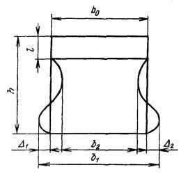
Fig. P2.1.
Sample breaking pattern
(b0
is a sample width; l is a cut depth; h is a sample height)
The applied
methods and criterial values of the viscous component in the fracture shall be
agreed by the testing organization with the leading material organization.
5.4.3.5. Lateral
expansion ∆b of the impact sample is the residual (plastic) deformation
on the edge opposite to the cut and measured in the direction of the cut, as
shown in Fig. P2.1, and determined by the formula.
∆b = b1
- b0 = ∆1 + ∆2.
The lateral
expansion is determined on the halves of the samples destroyed after impact
bending tests. Measurements of lateral expansion shall be made with an error of
± 0.01 mm.
5.4.3.6. The
arithmetic mean values of impact strength and the minimum values of viscous component
in the fracture and lateral expansion are determined according to the data
obtained from testing three samples at each test temperature. In the graphs in
the coordinates, the impact strength-temperature, the viscous component in the
fracture-temperature and the lateral expansion-temperature cause the indicated
values and successively connect them with straight lines. Here, values of
impact strength, fibrous of fracture and lateral expansion are plotted by the
points for each of the tested samples. The obtained graphs are the initial
information for determining the critical brittle temperature.
5.5. DETERMINATION OF THE CRITICAL BRITTLE
TEMPERATURE
5.5.1. The
temperature for which the following conditions are met is assumed as the
critical brittle temperature Tc.
5.5.1.1. At
temperature Tc, the arithmetic mean value of the impact
strength shall not be lower than the values indicated in Table P2.1, and
the minimum value of the impact strength shall not be lower than 70% of the
values indicated in Table P2.1.
Table P2.1. Criterial
values of the impact strength at temperature Tc, °C
|
Yield
limit at temperature of 20 °C Rр0.2, MPa
(kgf/mm2)
|
Impact
strength (KCV)I, J/cm2 (kgf · m/cm2)
|
|
Up to 304 (31)
inclusive
|
29 (3.0)
|
|
304 (31) to 402 (41)
inclusive
|
39 (4.0)
|
|
402 (41) to 549 (56)
inclusive
|
49 (5.0)
|
|
549 (56) to 687 (70)
inclusive
|
59 (6.0)
|
Table P2.2. Criterial
values of the impact strength at temperature Tc + 30, °C
|
Yield
limit at temperature of 20 °C Rр0.2, MPa
(kgf/mm2)
|
Impact
strength (KCV)II, J/cm2 (kgf · m/cm2)
|
|
Up to 304 (31)
inclusive
|
44 (4.5)
|
|
304 (31) to 402 (41)
inclusive
|
59 (6.0)
|
|
402 (41) to 549 (56)
inclusive
|
74 (7.5)
|
|
549 (56) to 687 (70)
inclusive
|
89 (9.0)
|
5.5.1.2. At
temperature (Tc +30) °С, the arithmetic mean value of the
impact strength shall not be lower than the values indicated in Table P2.2,
the minimum value of the impact strength shall not be lower than 70% of the
values indicated in Table P2.2, the minimum value of the viscous
component in the fracture shall not be lower than 50%.
5.5.2. If one of
the three tested samples fails to satisfy any of the conditions specified in
items 5.5.1.1 and 5.5.1.2, it is allowed to test three more
samples.
In this case,
when determining the compliance of the obtained results with the requirements
of items 5.5.1.1 and 5.5.1.2 use the showing of five samples,
except for the sample for which unsatisfactory results were obtained in the
first test.
5.5.3. If, during
additional tests specified in item 5.5.2, at least one sample shows
unsatisfactory indications, then the critical temperature Tc
is assumed to be the nearest high temperature at which the test results meet the
requirements of items 5.5.1.1. and 5.5.1.2.
5.5.4. If defects
are detected (in the form of cavities, delaminations, etc.) in the sample
fracture, it is allowed to exclude the results of its testing from
consideration and test a new sample.
5.5.5. The procedure
for processing test results is as follows.
5.5.5.1. According
to the known value of the material yield limit at a temperature of 20 °C is
selected according to Table P2.1 and P2.2 relevant criterial
values of the impact strength (KCV)I and (KCV)II. When
determining (KCV)I and (KCV)II for the fusion zone and
heat-affected zone of a welded joint, the yield limit of the base metal is
used.
The yield
limit is determined as the mean value of the test results of three or more
samples or as the maximum value if two samples were used in the tests.
5.5.5.2. On the
graph of the impact strength-temperature on the y-axis (KCV axis) the value of
(KCV)I is plotted. Through the obtained point, a line parallel to
the x-axis is drawn to the intersection with the impact strength curve.
The highest
test temperature nearest to the intersection point is assumed as the
temperature T1.
5.5.5.3. On the
graph of the impact strength-temperature on the y-axis the value of (KCV)II
is plotted. Through the obtained point, a line parallel to the x-axis is drawn
to the intersection with the impact strength curve.
The highest
test temperature nearest to the intersection point is assumed as the
temperature T'2.
5.5.5.4. On the
graph of the viscous component in the fracture-temperature on the y-axis the
value of B = 50 % is plotted. Through the obtained point, a line
parallel to the x-axis is drawn to the intersection with the curve plotted
based on the minimum values of the viscous component.
The highest
test temperature nearest to the intersection point is assumed as the
temperature T''2.
5.5.5.5. If, when
the requirements of items 5.5.5.2 - 5.5.5.4 are met, the lines
drawn parallel to the x-axis intersect the corresponding curves at two or more
points, then the temperatures T1, T'2 and T"2
shall be determined by the right extreme points of intersection.
5.5.5.6. Greater of
the temperatures T2 and T"2 is marked
as T2.
5.5.5.7. If the
difference between temperatures T2 and T1
is less than 30 °C, then the temperature T1 is assumed as an
indicative value of the critical brittle temperature T1c.
5.5.5.8. If the
condition of item 5.5.5.7 is not performed, then T1c
is determined by the formula T1c = T2
- 30 °C.
5.5.5.9. Additional
tests at temperatures (T1c ± 10) °C, (T1c
+ 20) °C, (T1c + 30) °C, (T1c
+ 40) °C are conducted, the impact strength curves and viscous component in the
fracture are specified, and in accordance with the instructions of items 5.5.5.2
- 5.5.5.8 the value of the critical brittle temperature is finally set
(if during the tests the values of KCV and B have already been
determined at the temperatures indicated in this item, additional testing at
these temperatures is not required).
5.5.6.
Confirmation of the critical brittle temperature can be carried out in cases
where its guaranteed value Tcr is specified in the regulatory
technical or design documentation. When the critical brittle temperature is
confirmed, tests are carried out in compliance with the requirements of this
procedure in the following sequence:
1) tests are
carried out at guaranteed temperature Tcr and temperature (Tcr
+ 30) °C;
2) compliance
with the conditions of item 5.5.1.1 at a temperature Tcr
and item 5.5.1.2 at a temperature (Tcr + 30) °C is
checked, and conditions of items 5.5.2 - 5.5.4 apply.
If conditions
1) and 2) are met, then the critical brittle temperature is considered
confirmed.
If
requirements of item 5.5.1.2 are met at temperature Tcr,
then it is allowed not to perform tests at temperature of (Tcr
+ 30) °C.
If
requirements of items 5.5.1.1 and 5.5.1.2 at temperatures Tcr
and (Tcr + 30) °C are not met, then the critical brittle
temperature is considered unconfirmed.
6. PROCEDURE FOR
DETERMINING CRITICAL BRITTLE TEMPERATURE SHIFT DUE TO THERMAL AGEING
6.1. GENERAL
6.1.1. The
critical brittle temperature shift due to thermal ageing is determined by the
formula
∆Tt
= Tct – Tc0,
where Tct
is a critical brittle temperature of the material subjected to heat ageing; Tc0
is a critical brittle temperature of the material in the initial state (before
ageing).
6.1.2. Definition
of values of Tc0 and Tct is carried out in accordance
with the instructions of Section 5 of this Appendix.
6.1.3. Sample
collection, requirements for samples and their preparation and orientation in
the studied semi-finished product shall meet the instructions of Section 5
of this Appendix.
6.2. PERFORMING OF TESTS AND PROCESSING OF RESULTS
6.2.1. Thermal
ageing is carried out on blanks with a size of at least 60×13×13 mm.
6.2.2. Temperature
of thermal ageing is set in accordance with the regulatory and technical
documentation for the product or material; it shall not be less than the design
temperature or exceed it by more than 100 °C.
6.2.3. In the
process of holding the samples during thermal ageing, a temperature fluctuation
within ± 5 °C from the nominal value of the ageing temperature is allowed.
6.2.4.
Preparations of samples for impact bending tests are maintained at a given
temperature for 500, 1000, 3000, 5000, 7500 and 10000 hours.
For steels
that do not have an extremum of changes in Tct in the process
of ageing with a holding of 5000 to 10000 hours, it is allowed not to carry out
tests with a holding time of 7500 hours.
6.2.5. According
to the results of impact bending tests of samples cut from blanks that were
subjected to aging for various periods of time, the value of Tct
is determined and, in accordance with item 6.1.1, the values of ΔTt
on the bases specified in item 6.2.4 are also determined.
6.2.6. If the
values of ∆Tt for all time intervals are negative, the design
value of ∆Tt is assumed to be equal to zero.
6.2.7. In the case
of a monotonous, saturation tending change in the dependence of Tct
on the ageing time, the experimental data of ΔTt = Tct
- Tc0 for different duration of ageing are approximated by
the equation
∆Tt
= ∆Ttlim[1 - exp(-pt)],
where ∆Ttlim,
p are empirical constants determined using mathematical statistics
methods; t is ageing time.
A design value
of ΔTt means the value of ΔTtlim
if the difference between ΔTtlim and a
shift obtained by the formula of this item based on 10000 hours does not exceed
10 °C. Otherwise, the design value of ∆Tt for the operation
duration of not more than 100000 hours shall be determined by the formula of
this item. If extrapolation is necessary for a longer period, the ageing
duration shall be increased. In this case, extrapolation is allowed to be
carried out for a time not exceeding a tenfold maximum duration of ageing.
6.2.8. With the
extreme nature of the dependence of Tct on the ageing time in
the time intervals according to item 6.2.4, the approximation of the
falling section of the dependence is used by the equation
∆Tt
= ∆Ttmaxexp[-b(t – tmax)]
+ c,
where ∆Ttmax
is a critical brittle temperature shift in the field of extremum; t is
an ageing time at which extremum (maximum) is observed; b, c are
empirical constants determined using mathematical statistics methods.
6.2.9. If at the
temperature and duration of ageing according to items 6.2.2 and 6.2.4
there is a monotonous increase in Tct, not tending to
saturation, it is allowed to establish the dependence of Tct
on the ageing time using the Hollomon parameter by the formula
Нр = (T + 273)(k
+ lgt) · 10-3,
where t is an
ageing duration, h; T is an ageing temperature, °C; k is an
empirical constant determined by the mathematical statistics methods.
In this case,
the aging temperature shall exceed the one specified in item 6.2.2 by 50
°C, and the aging duration shall be 1000, 3000, 5000 hours.
The procedure
indicated in this item is applicable provided that the same way of change of
dependencies of Tct at the ageing temperatures used.
7. PROCEDURE
FOR DETERMINING CRITICAL BRITTLE TEMPERATURE SHIFT DUE TO FATIGUE DAMAGE
ACCUMULATION
7.1. GENERAL
7.1.1. The
critical brittle temperature shift due to fatigue damage accumulation is
determined by the formula
∆TN
= TcN - Tc0,
where TcN
is a critical brittle temperature of the material subjected to cyclic loading; Tc0
is a critical brittle temperature of the material in the initial state (before
cyclic loading).
7.1.2. Definition
of values of TcN and Tc0 is carried
out in accordance with the instructions of Section 5 of this Appendix.
7.1.3. Sample
collection, requirements for their preparation and orientation in the
semi-finished product shall meet the instructions of Section 5 of this
Appendix.
7.1.4. The TcN
is determined according to the results of impact bending tests of samples cut
from the working part of the base samples.
7.2. TESTING
7.2.1. To assign
the cyclic loading modes of the base samples, the fatigue curve of the material
under study is used in the range of 103 ... 104 cycles,
obtained at hard loading.
The design
definition of fatigue curves is allowed without the introduction of safety
coefficients for stresses and number of cycles using the actual strength and
ductility characteristics of the material under study.
7.2.2. Base
samples prepared of the material under study are subjected to cyclic loading at
a temperature of (20 ± 5) °C. Before loading the base samples, the critical
brittle temperature of the material under study in the initial state is
determined.
7.2.3. For
cyclically softening materials (with a ratio of RTp0.2/RTm
> 0.7), cyclic loading of the base samples is carried out under axial
tension in the soft mode with the cycle asymmetry coefficient on the load r
@ 0.05 up to the accumulation of residual axial deformation (2.5 ± 0.25) %. In
this case, the stress shall correspond to a value that ensures accumulation of
the required residual deformation for at least 103 cycles.
It is allowed
to apply the loading of base samples by bending in a soft mode with an
asymmetry coefficient r @ 0.05. At the same time, in the cutting area of
finished impact samples (at the cut section) located only in the zone of
residual tension deformations, the deformation of the metal of the base samples
shall be at the level of (2.5 ± 0.25) %. The cut on the impact sample shall be
located on the side of maximum plastic deformation.
7.2.4. For
cyclically stable and cyclically hardening materials (with a ratio of RTp0.2/RTm
≤ 0.7) the purpose of loading modes of the base samples is made on the basis of
the low-cycle fatigue curve of the material under study at a symmetric cycle
according to item 7.2.1, determining the amplitudes of the conditional
elastic stresses (deformations) corresponding to the numbers of cycles 103
and 104. At the specified amplitudes of stresses (deformations),
loading of the base samples is carried out until fatigue damage accumulation a
is not less than 0.3.
It is allowed
to load the base samples by alternating bending (r = -1), while within
the sizes of the finished samples (at the cut) the amplitude of deformations
shall not differ by more than 10%. The cut on the impact sample shall be
located in the place of the greatest value of the amplitude of deformations.
7.2.5. The design
shift of the critical brittle temperature is determined in accordance with item 7.1.1
and is assumed to be equal to the largest value obtained in the considered
range of numbers of loading cycles, stresses (deformations). If it turns out
that ∆TN < 0, then ∆TN = 0 shall be
assumed as a design characteristic.
8. PROCEDURE FOR
DETERMINING CRITICAL BRITTLE TEMPERATURE SHIFT DUE TO EFFECTS OF EXPOSURE
AND RADIATION EMBRITTLEMENT COEFFICIENT
8.1. GENERAL
8.1.1. The
critical brittle temperature shift due to exposure effect is determined by the
formula
∆TF = TcF
- Tci,
where ∆TF
≥ 0; TcF is a critical material brittle temperature
after exposure; Tci is a critical material brittle
temperature in the initial state (before exposure).
8.1.2. The
radiation embrittlement coefficient is determined from the ratio
AF = ∆TF(Fn/F0)n,
where Fn
is a neutron transfer with an energy of Е > 0.5 MeV; F0
= 1022 neutron/m2; n is a coefficient.
8.2. EXPOSURE OF SAMPLES
8.2.1. Samples can
be exposed both in research and in power reactors, both in dry ampoules and in
coolant flow.
8.2.2. Witness
samples loaded into the body of a nuclear power reactor are placed in sealed
containers bound together in a bunch.
8.2.3. When
exposing samples loaded into the reactor in sealed ampoules, reliable heat
removal from the sample using fillers (aluminum, helium, sodium or others)
shall be ensured.
8.2.4. The
temperature deviation from the point set during exposure in a steady-state mode
shall not exceed ±10 °C.
8.2.5. When exposing
samples in sealed ampoules, continuous temperature control shall be carried out
by thermocouples attached to the samples by spot welding on their surface or
pressed into the sample. The distance between thermocouples is determined by
the design of the irradiation device, but shall not be more than 200 mm.
Control over
the temperature change during the exposure process shall be carried out
automatically with recording on the recorders. The error of indication shall be
no more than ±5 °C. It is recommended to install the maximum exposure
temperature fixation indicators, which shall be installed directly on the
samples.
If it is
impossible to install thermocouples under exposure in power reactors, it is
allowed to control the maximum exposure temperature only with the help of
diamond monitors or fusible thermal indicators.
8.2.6. When
exposing samples in unsealed ampoules, the exposure temperature is controlled
by the coolant temperature at the inlet and outlet of the nuclear core or
process channel.
8.2.7. The flux
density of fast neutrons with an energy of E ≥ 0.5 MeV along the height
of the placement of samples intended to determine ∆TF at the
selected value of neutron transfer shall not differ by more than 15%.
8.2.8. The
transfer of fast neutrons affecting the samples is determined using activation
indicators. The number of indicators and the distance between them in the
radial and axial directions of the irradiation device is selected depending on
its geometry and size, but at least three (in the center and along the edges).
The error in determining the neutron transfer shall be no more than ± 15% of
the measured value.
8.2.9. The
exposure report shall contain the following data:
1)
nomenclature and order of placement of samples in the reactor;
2) energy
spectrum of neutrons at the location of the samples in the reactor;
3) records of
temperature of samples during exposure, type of thermocouples and method of
their fastening;
4) temperature
distribution along the height of the irradiation device for the entire period
of exposure;
5) type of
indicators for determining neutron transfer and their distribution along the
cross section and height of the irradiation device;
6) schedule of
reactor operation with shutdowns for planned preventive maintenance (PPM);
7) pressure,
temperature, speed and chemistry of the coolant and their change in the process
of exposure of samples;
8) time of
exposure of samples reduced to 100% reactor power.
8.2.10. After
exposing the samples in contact with the coolant, a conclusion shall be made
about their appearance, the content and distribution of hydrogen in the samples
shall be analyzed, and a conclusion about the corrosion effect of the coolant
on the sample material shall be made.
8.3. PERFORMING OF TESTS AND PROCESSING OF RESULTS
8.3.1. Impact
bending tests for samples from materials in the initial and exposed states
shall be carried out on the same equipment.
8.3.2. The number
of samples for testing the material in one state (exposed or unexposed) shall
correspond to the number of samples required to determine the critical brittle
temperature according to Section 5 of this Appendix. In the case of a
limited number of samples due to an insufficient amount of devices for
exposure, it is allowed to use the test data of a smaller number of samples,
but not less than 12, to make a single temperature dependence KCV.
8.3.3. If the
number of exposed specimens of the same series (with one fluence) is
insufficient (due to the reasons specified in item 8.3.2) to determine
the critical brittle temperature in full accordance with the instructions in
Section 5 of this Appendix, the processing of experimental data from
tests of exposed and unexposed samples is carried out in the following way:
1. Plot a
graph of impact strength dependence (KCV) on the test temperature T
using the equation
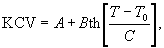
where A is a mean
value of KCV between upper KCVmax and lower KCVmin
values of impact strength; B = (KCVmax – KCVmin)/2;
T0 is a temperature corresponding to the value of A; C
is an empirical constant.
Values of A,
B, C and T0 are determined by processing the
experimental data by the least square method.
Experimental
values of impact strength are plotted on a graph for each of the tested
samples.
The graphs
obtained by the above equation are the initial information for determining the
critical brittle temperature.
2. According
to the known value of the yield limit of the material in the initial state
(when determining the value of Tсi) or after exposure (when
determining the value of TсF) at a temperature of 20
°C in accordance with the values given in Table P2.1, the criterial
value of impact strength is selected (KCV)I. In this case, each of
the values of the yield limit indicated in the table is assumed as an mean
value if at least three samples were used to determine it, and as a maximum
value if two samples were used to determine it.
3. On the KCV-T
graph on the y-axis (KCV axis) the value of (KCV)I is plotted.
Through the obtained point, a line parallel to the x-axis (temperature axis) is
drawn to the intersection with the impact strength curve.
Temperature
corresponding to the intersection point is indicated as T1.
4. On the KCV-T
graph on the y-axis the value 1.5(KCV)I is plotted. Through the
obtained point, a line parallel to the x-axis is drawn to the intersection with
the impact strength curve.
Temperature
corresponding to the intersection point means the temperature T2.
5. If the
temperature difference T2 - T1 is less than
30 °C, then temperature T1 is assumed as a value of Tci
or TcF (for the initial and exposed states,
respectively).
6. If
condition 5 is not met, then the value of T2 - 30 °C is
assumed as Tci or TcF.
9. FATIGUE TEST METHODS
9.1. GENERAL
9.1.1. The terms
and definitions used when conducting fatigue tests and processing experimental
data are set in accordance with GOST 23207-78.
9.1.2. Determined
fatigue resistance characteristics are used for:
1) obtaining
characteristics of fatigue fracture resistance of structural materials and
their welded joints used in calculations for cyclic strength according to these
regulations;
2) comparison
of materials and their welded joints of various chemistry, their manufacturing
technology and quality;
3)
justification of the selection of materials for the considered components of
equipment and pipelines.
9.1.3. The main
characteristics to be determined from the results of testing metals and their
welded joints for cyclic strength (fatigue) in low-cycle and high-cycle areas
are:
1) static and
cyclic deformation diagram before deformations of at least 3% and constants of
the equations of deformation curves at their power approximation;
2) fatigue
curves under loading with given deformations and constants of the equations of
fatigue curves at their power approximation;
3) fatigue
curves under loading with given forces and constants of the equations of
fatigue curves at their power approximation;
4) material
endurance limit for a given number of cycles under symmetric loading;
5)
coefficients of reduction of cyclic strength of the welded joint, and the metal
with deposit welding φs;
6) curves of
long-term cyclic strength of structural materials and their welded joints;
7) coefficient
of reduction of cyclic strength of structural materials and their welded
joints, with due regard to the effect of neutron exposure;
8)
coefficients of reduction of cyclic strength of structural materials and their
welded joints, with due regard to the effect of the corrosive environment.
9.1.4. The basic
requirements for experimental equipment, for the shape and size of samples, for
their preparation and surface cleanliness are set in accordance with GOST
25.502-79.
9.1.5. The shape
and size of test samples are selected with due regard to the shape and size of
the sections of blanks for the components of NPI equipment and pipelines, as
well as the test objectives.
For rod and
sheet components of equipment with a wall thickness of over 20 mm,
predominantly cylindrical samples are used; and for thin-walled sheet
components of equipment with a wall thickness of up to 10 mm, flat samples are
used.
9.1.6. Deformation
of the working part of samples of types II and IV according to GOST 25.502-79
is measured by longitudinal deformometers, and the distance from the
deformometer supports to the transition part shall be at least 2 mm.
9.1.7. When
testing samples of types I and III according to GOST 25.502-79, transverse
deformometers are used.
Longitudinal
deformation is determined by the formulas
 or
or 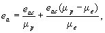
where eapc,
eaec are amplitudes of plastic transverse and elastic
transverse deformations, respectively; eac, eae
are amplitudes of elastic plastic transverse and elastic longitudinal
deformations, respectively; μp, μe is a
Poisson ratio for plastic and elastic deformations, respectively. It is allowed
to assume that μp = 0.5 and μe = 0.3.
9.1.8. When
conducting fatigue tests at elevated temperatures, the error in maintaining and
measuring the set temperature of the working part of the sample shall not
exceed ±5 °C in the temperature range from 50 to 600 °C.
9.1.9. Equipment
for heating samples shall provide heating of the working part of samples of
types II and IV (for samples of types I and III, section with radius R)
according to GOST 25.502-79 with temperature differences along the length and
diameter (thickness) of not more than 5 °C per 10 mm.
9.1.10. For material
tested for fatigue, the characteristics of short-term and long-term static
strength and ductility at appropriate test temperatures and loading duration
shall be obtained according to Section 2 of this Appendix and Appendix
6.
9.2. LOW-CYCLE FATIGUE
9.2.1. The main
mode of low-cycle loading of samples is axial tension-compression with given
deformation amplitudes.
Bending or
torsion testing is allowed.
9.2.2. For
materials prone to cyclic softening (with a ratio of yield limit to tension
limit of above 0.7), along with the tests specified in item 9.2.1, tests
with a given amplitude of stresses (forces) shall be carried out.
9.2.3. The
characteristics of low-cycle fatigue resistance specified in item 9.1
are determined from the results of test of a series of samples, which shall be:
1) at least
three – to determine the deformation diagrams;
2) not less
than ten – to determine the fatigue curves for the formation of cracks with a
length of over 0.5 to 2.0 mm with a symmetric cycle of deformations or
stresses.
9.2.4. With the
tendency of samples of type II and IV according to GOST 25.502-79 to loss
stability, the length of the working part l of samples of type II is allowed to
be reduced to 2d (d is a working part diameter) and of type IV to
 (b
is a height; h is a thickness of a working part of the flat sample).
(b
is a height; h is a thickness of a working part of the flat sample).
9.2.5. Tests for
low-cycle fatigue are carried out in the air:
1) with axial
tension-compression (the main type of loading);
2) with
amplitudes of stresses above the yield limit and corresponding deformations;
3) with a
symmetric cycle on a controlled parameter (deformation or stress);
4) with a
number of loading cycles of 102 to 5 · 104 (at least);
5) with a
loading frequency of up to 1 Hz, which excludes self-heating of samples by more
than 30 °C.
9.2.6. Testing
procedure:
1) inspection
and measurement of the cross-sectional sizes of the working part of the samples
with an error of no more than 0.5% of the nominal size;
2) static
tests to determine the mechanical properties;
3) zero
half-cycle of loading the samples under tension;
4) the first
sample is tested at a deformation amplitude of 1% (under loading with given
deformations) and a zero half-cycle deformation of 0.6% (under loading with
given loads);
5) subsequent
samples, depending on the test result of the first sample, are tested at the
deformation amplitudes or zero half-cycle deformations, ensuring an
approximately uniform distribution (on a logarithmic scale) of the resulting
durabilities in a given range of cycle numbers according to item 9.2.5;
6) during the
test, recording of loads and deformations is carried out on an x-y recorder in
a zero half-cycle and in cycles of 10p, 2 · 10p,
3 · 10p, 5 · 10p, where p = 0, 1, 2,
3, 4.
When
conducting a test to determine the durability, the number of cycles is
recorded, corresponding to the moment of crack formation according to item 9.2.3.
9.2.7. According
to the test results of a series of samples, a summary protocol is drawn up that
includes the input data (material grade; heat treatment; type of blank;
location and orientation of the sample cutting; shape, size and labeling of the
sample; type of machine; test conditions) about the series of samples, data on
the amplitudes of deformations, stresses, durability to crack formation, and
constants of the equations of deformation diagrams.
9.2.8. The test
results under loading with given deformation amplitudes of each sample of the
series are represented graphically in double logarithmic coordinates:
1) lgea
– lgN;
2) lgeap
– lgN;
3) lgeae
– lgN.
The above
deformation amplitudes are accepted for a stabilized cycle or a number of
cycles equal to 0.5N.
9.2.9. The test
results under loading with given stress amplitudes of each sample of the series
are represented graphically in coordinates lgeap –
lgN. In this case, the amplitude of plastic deformations eap
is set by calculation on the zero half-cycle deformation е0
by the formula
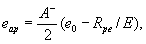
where Rpe
is a limit of proportionality in zero half-cycle, MPa; E is a modulus of
elasticity, MPa;  is a
coefficient characterizing the relationship between the deformation e0
and hysteresis loop width δ1 in the first half-cycle of loading and
assumed to be equal to the mean value of the set of experimental values A
of a series of samples according to item 9.2.3, determined by the
formula
is a
coefficient characterizing the relationship between the deformation e0
and hysteresis loop width δ1 in the first half-cycle of loading and
assumed to be equal to the mean value of the set of experimental values A
of a series of samples according to item 9.2.3, determined by the
formula
A = δ1(e0
– Rpe/E).
9.2.10. The fatigue
curves according to the experimental points are plotted by the of least square
method.
In cases of
determining only the amplitudes of elastics plastic deformations ea
(without separating them into elastic and plastic components) fatigue curves
can be plotted by graphical interpolation.
9.2.11. The
design characteristics are determined by the fatigue curves:
1) according
to items 9.2.8 and 9.2.10 in plastic deformations
eap(4N)m
= ec,
where m, ec
are the constants of equations, which are recorded in the summary test report;
2) according
to items 9.2.8 and 9.2.10 in elastic deformations
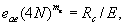
where mе,
Rc are the constants of equations, which are recorded in the
summary test report;
3) according
to items 9.2.9 and 9.2.10 in plastic deformations

where m1,
ecb are the constants of equations, which are recorded in the
summary test report.
9.2.12. The cyclic
deformation diagram is obtained according to the test data at a given
deformation amplitudes for a stabilized cycle or a number of cycles equal to
0.5 of durability in the coordinates of "deformation amplitude 2ea
– stress range 2σa.
9.2.13. The cyclic
deformation curve hardening rate in the inelastic section is obtained by
plotting a deformation curve in the double logarithmic coordinates lg(2σa)
- lg(2ea) as a slope of the approximation straight
line:
2σa = (2Rpe)1
- v – (2Eea)v.
The summary
test report records the value of the hardening rate v, obtained as an
arithmetic mean for at least three samples.
The static
deformation diagram is drawn similarly with the replacement of 2σa,
2ea, 2Rpe to σ0, e0,
Rpe (stress and deformation of the zero half-cycle,
respectively).
9.3. MULTICYCLE FATIGUE
9.3.1. The
multicycle fatigue characteristics in a given range of amplitudes of stresses
(deformations) and at a given asymmetry are obtained from the results of tests
of a series of samples, which number shall be at least 12.
9.3.2. The shape
and size of test samples are selected with due regard to the shape and size of
the sections of blanks for the equipment components and test objectives.
For rod and
sheet components of equipment with a wall thickness of over 20 mm,
predominantly cylindrical samples are used; for thin-walled components of
equipment with a wall thickness of up to 10 mm, flat samples are used.
9.3.3. The main
mode of a multicycle loading of samples is axial tension-compression.
9.3.4. Tests for
multicycle fatigue are carried out in the air:
1) with axial
tension-compression (the main type of loading);
2) with a
symmetrical loading cycle;
3) with the
number of loading cycles for steels above 5 · 104 to 107;
4) with a
loading frequency of up to 200 Hz, which excludes self-heating of samples by
more than 30° from a given temperature.
9.3.5. When
assessing the material sensitivity to the cycle asymmetry, in addition to tests
with an asymmetry coefficient rσ (re) = -1,
tests are carried out in the scope specified in item 9.3.1, at values rσ
(re) = 0, where
rσ = σmin/σmax (re
= emin/emax);
σmin(emin)
is a minimum stress (deformation) of the loading cycle; σmax(emax)
is a maximum stress (deformation) of the loading cycle.
9.3.6. It is
allowed to carry out bending tests with rotation of samples of circular
cross-section of types I and II according to GOST 25.502-79, with flat bending
of samples of types III and IV in accordance with GOST 25.502-79, and during
torsion of samples of circular cross-section for the corresponding type of
loading of the component of structure.
9.3.7. Testing
procedure:
1) inspection
and measurement of the cross-sectional sizes of the working part of the sample
with an error of no more than 0.5% of the nominal size;
2) the first
sample is tested at a stress amplitude of (0.6 ÷ 0.65)RTm
(when loading with a constant amplitude of total deformation, this amplitude
shall be assumed to be equal to 0.4 %);
3) the
subsequent samples (approximately 2/3 of the remaining amount), depending on
the test result of the first sample, are tested with amplitudes of stresses
(deformations) ensuring an approximately even distribution of the obtained
durabilities N before crack formation with a length of 0.5 to 2 mm in
the specified range of the number of cycles specified in item 9.3.4;
4) test
results are pre-processed and a fatigue curve is obtained;
5) to
determine the endurance limit based on tests of 107 cycles, at least
three samples are tested at a stress amplitude assumed according to a
preliminary fatigue curve. If two samples of the three tested or at least half
of the tested samples are not destroyed until the specified number of cycles is
reached, then this amplitude is assumed to be the endurance limit;
6) the
obtained endurance limit is tested by testing one sample with an amplitude of
0.95 of the endurance limit, and the sample shall not be destroyed at a
specified number of cycles;
7) the test
results are finally processed and the characteristics of multicycle fatigue are
determined, while the experimental point closest to the endurance limit shall
be obtained with an amplitude of no more than 1.05 of the endurance limit.
9.3.8. Based on
the test results, a summary protocol drawn up that includes the input data
(material grade; heat treatment; type of blank; location and orientation of the
sample cutting; shape, size and labeling of the sample; test conditions) about
the series of samples, data on the amplitudes of stresses (deformations) and
durability.
9.3.9. The test
results of each sample are presented graphically in double logarithmic
coordinates lgσa – lgN.
9.3.10. The fatigue
curves according to the experimental points are plotted by the of least square
method.
9.3.11. According
to the fatigue curve, the design characteristics are determined – the endurance
limit on a given base and the exponent me of the fatigue
curve:
where N0
is a given number of cycles (test base).
9.3.12. According
to the test results at an asymmetric cycle according to item 9.3.5, the
sensitivity coefficient of the material to the asymmetry of the stress
(deformation) cycle is determined by the formula
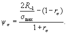
9.4. LONG-TERM CYCLIC STRENGTH
9.4.1. Tests for
long-term cyclic strength are carried out according to GOST 25.505 - 85
"Calculations and tests for strength. Methods mechanical tests of metal.
Tests at low-cycle non-isothermal and thermal fatigue loading on the basis of 2
· 104 h at a temperature that causes the greatest decrease in the
long-term plasticity of the material under study. Characteristics of long-term
strength and ductility are determined in accordance with the requirements of
Section 4 of this Appendix.
9.4.2. The main
type of loading is axial tension-compression with given deformation amplitudes.
Bending tests
with a given displacement are allowed.
9.4.3. The tests
are carried out before the crack formation with a length of over 0.5 to 2 mm:
1) in the
low-cycle area (102 - 104 cycles) with a symmetrical
loading cycle (re = -1);
2) in the
high-cycle area (105 - 107 cycles) with a symmetric and
pulsating (rσ = 0) loading cycles.
9.4.4. The loading
frequency and holding time at maximum cycle deformation are assumed such that
the maximum test duration within a given series of samples on an accepted cycle
base is at least 10% of the operation time of a component of structure made of
the material under study.
9.4.5. The number
of samples within one series shall be at least eight (by two samples at four
levels of deformation amplitudes).
9.4.6. The test
results are presented in the form of fatigue curves according to the endurance
duration parameter. It is allowed to plot fatigue curves according to the
experimental points by graphic interpolation.
9.4.7. The design
characteristics of long-term cyclic strength are determined using the
recommendations of Appendix 7 of the Regulations.
9.4.8. According
to the test results at an asymmetric cycle according to item 9.4.3, the
sensitivity coefficient of the material to the asymmetry of the loading cycle
is determined using the formula in item 9.3.12.
9.5. CYCLIC
STRENGTH OF WELDED JOINTS AND METAL WITH DEPOSIT WELDING
9.5.1. Fatigue
tests of metal of various zones of welded joints and metal with deposit welding
are carried out in accordance with the requirements of GOST 25.502-79, GOST
25.505-85 and items 9.1 - 9.4.
9.5.2. When
testing a welded joint metal, the longitudinal axis of samples of types II, IV
according to GOST 25.502-79 shall be placed parallel to the welded joint axis.
It is allowed to use samples of types I and III with the location of the sample
axis perpendicular to the welded joint axis.
For the
preparation of samples, welded joints of the first category are used.
9.5.3. When
testing metal of transition zones (fusion zone and heat-affected zone) the
minimum cross-section of samples of types I, III according to GOST 25.502-79
shall be placed in the test zone of the welded joint. According to the test
results, the fatigue curve is plotted, which is the lower envelope of the
curves of the various zones of the welded joint.
It is allowed
to obtain a fatigue curve using samples of types II and IV with the location
within the measurement base of the longitudinal deformation of all zones of the
welded joint.
9.5.4.
Characterization of the cyclic strength of the metal with deposit welding is
carried out on samples with the preservation of a deposit welding in full size.
The height of the sample is assumed to be H = 4B, where B
is an overlay thickness. For single-layer deposit welding, the use of samples
with a smaller section of the working part is allowed. In this case, the
overlay thickness shall be at least (2 ± 0.5) mm.
9.5.5. To
determine the diagram of cyclic deformation of the deposited metal, a sample
entirely cut out of the overlay metal is used.
9.5.6. If, when
testing metal of transition zones of welded joints, cyclic fractures do not
occur in the sample zone under study, then the sample zone under study is
transferred to the part where the fractures occur.
9.5.7. When
testing flat samples with deposit welding, the zone in which cracks occur
(overlay, sub-surfacing zone, base metal) is fixed.
9.5.8. According
to the results of fatigue tests of the base metal in accordance with the
indicated in items 9.2 - 9.4, as well as the metal of welded
joints and metal with deposit welding, the coefficient of reduction of the
cyclic strength of a welded joint or metal with deposit welding φs
is determined at a given durability N by the formula
φs
= eas/ea,
where eas
is a deformation amplitude according to the fatigue curve of the welded joint; ea
is a deformation amplitude according to the fatigue curve of the base metal.
9.5.9. To
determine the values of φs, the curves ea -
N obtained according to items 9.5.3, 9.5.4 are used. If
the obtained value is φs > 1, then it is assumed that φs
= 1.
If in the
interval of numbers of cycles 102 - 107 the difference of
φs from φs at N = 104 is
not more that by ±10 %, then the minimum value of φs, set
according to the curve φs - N is assumed. In other
cases, the values of φs are determined by dependency φs
– σa(ea), which is used in the
calculations.
9.5.10. The results
of cyclic tests of the metal of welded joints and metal with deposit welding
are recorded in the summary test report.
9.6. CYCLIC STRENGTH OF BASE MATERIALS, WELDED
JOINTS AND METAL WITH DEPOSIT WELDING IN CORROSION MEDIA
9.6.1. When
testing for cyclic strength, the following design characteristics are
determined:
1) fatigue
curves at low-cycle loading in the amplitudes of elastic plastic deformations
in air and in a medium at a given temperature, cycle form, and loading
frequency;
2) φc
(φcs) is a coefficient of corrosion reduction of the cyclic
strength of the base metal (welded joint), equal to the ratio of the value of ea
according to the fatigue curve obtained when testing in the medium to the value
ea according to the fatigue curve obtained when testing
samples of the same type in the air, with durability N;
3)  is a
minimum value of the coefficient of corrosion reduction of cyclic strength φc
(φcs).
is a
minimum value of the coefficient of corrosion reduction of cyclic strength φc
(φcs).
In the
following, only φc and  are used.
9.6.2. The
coefficients of corrosion reduction of cyclic strength are determined from the
results of tests of a series of samples in air and in a corrosive medium under
identical conditions of test temperature, material and dimensions of the
working part of the sample.
9.6.3. When
testing, samples of types I - IV according to GOST 25.502-79 are used. For
axial tension-compression or torsion, the tubular sample indicated in Fig. P2.2
is used.
When loading
with a pure or cantilevered bending, samples, the working part of which is
shown in Fig. P2.3, P2.4, are used. The design of transition
zones shall exclude destruction within them.
9.6.4. When
testing samples containing the fusion zone within the working part, the
measurement and control of deformation are carried out, as for a homogeneous
metal.
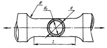
Fig. P2.2.
Sample for axial tension-compression and torsion tests:
(d - d1)/d
= 0.05 ÷ 0.1; d – d1 ≥ 1 mm; R ≥ d; l
= (3 ÷ 4)d. For tension-compression samples l/d is
determined by sustainability requirements
9.6.5. The number
of samples and the requirements for their preparation are specified in item 9.2
of this Appendix.
9.6.6. Samples are
labeled at both ends in such places and in such a way as not to reduce the
resistance to cyclic fracture and to ensure the labeling security after the
test.
9.6.7. The sample
is tested in the state corresponding to the state of the metal of the
manufactured or operated product.
9.6.8. In the
study of mechanisms of corrosion and fatigue destruction it is allowed to
pretreat the samples:
1)
autoclaving;
2) air
oxidation at elevated temperatures;
3) holding at
elevated temperature with or without prior plastic deformation;
4)
sensitization heating of the sample blanks in the study of the welding cycle
influence on the base metal in the heat-affected zone.
9.6.9. With axial
tension-compression of samples, measurement and control of deformations are
determined in accordance with GOST 25.502-79.
9.6.10. The
deformation amplitude on the surface of the working part of the sample from a
homogeneous material with a constant rectangular cross section under loading
with pure (four-point) bending is determined by the formula.
ea = ∆a8s/l2p,
where ∆a
is an amplitude of the movement of the middle of the working part relative to
the middle supports, mm; s is a height of the cross section of the
working part of the sample, mm; lp is a length of the working
part of the sample (the distance between the middle supports), mm.
The scheme of
loading with a pure bending is shown in Fig. P2.5.
When testing a
sample of a homogeneous or non-uniform material (for example, including various
zones of a welded joint), the amplitude of deformations in the working part of
the sample can be determined experimentally, for example, using strain
measurement.
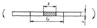
Fig. P2.3.
Working part of the sample for pure bending tests:
s ≥ 2 mm; lp
≥ 7s; 1.5 ≤ b/s ≤ 2.5
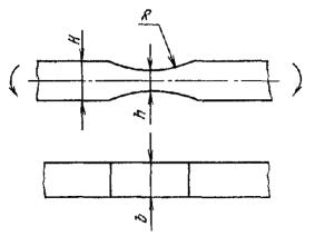
Fig. P2.4. The
shape and dimensions of the working part of the sample for
cantilevered bending tests:
|
h, mm
|
b, mm
|
H/h
|
R/h
|
|
2 - 10
|
(2 - 10)h
|
1.5 - 2
|
≥ 5
|
9.6.11.
Deformation of the working part of the sample is allowed to be determined by
the grip displacement outside the autoclave using the calibration dependencies
obtained when tested in air.
9.6.12. Testing
equipment includes a circuit filled with a medium and a loading device, which
can be a universal or special testing machine that maintains a given loading
mode, shape and characteristics of the cycle.
9.6.13. Test
equipment shall provide:
1) measurement
of displacements with an error of not more than ± 3% of the specified value;
2) the error
of maintaining cyclic displacements shall not exceed ±5% of the specified
values;
3) the error
of maintaining and measuring the set temperature shall not exceed ±5 °C in the
temperature range of 20-350 °C;
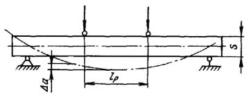
Fig. P2.5. The
scheme of loading a prismatic sample with pure bending
4) control and
maintenance of pressure with an error of no more than ± 5% of the specified
value;
5) control and
maintenance of the medium by pH = 4.5 ÷ 10.5, content of Cl (up to 10 µg/kg)
and O2 (up to 10 mg/kg) ions, as well as other by components
introduced into the composition of the real working medium, for example, when
boring or regulating the oxygen content with an error of no more than ± 10% of
the specified value;
6) forced
circulation of the medium (tests are allowed at natural circulation);
7) fixing the
moment of a crack occurrence with a length of 0.5–2 mm or the destruction of
each sample in the process of testing machine operation.
9.6.14. Tests are
conducted:
1) when
pulsating and symmetric deformation cycles with axial tension-compression or torsion
of cylindrical and tubular samples, pure or cantilevered bending of flat
samples. Only tests on a pulsating cycle are allowed;
2) with a
number of loading cycles of 102 to 5 · 104;
3) in the air
and in the corrosive medium at the same temperatures (at the maximum
temperature of the working medium without fail). Frequency (speed) of loading
in air is determined by the requirements of GOST 25.502-79;
4) in air in
accordance with GOST 25.502-79;
5) in a medium
with holding ∆t0 at a maximum tension deformation (∆t0
≥ 30 c). (φc)0 and  are determined at N
= 102, 103, 104, 5 · 104;
are determined at N
= 102, 103, 104, 5 · 104;
6) the
following tests for cyclic strength in the medium are carried out with
increasing holding of ∆tn = m∆t0, where m
= 5, 10, 50, ..., and correspondingly n = 1, 2, 3, ...;
7) tests are
terminated if the condition 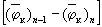 is met and the
graphs of dependencies (φc)m on lg(∆τm)
at values of N = 102, 103, 104, 5 · 104
note a decrease in the rate of decrease (φc)m,
that is
is met and the
graphs of dependencies (φc)m on lg(∆τm)
at values of N = 102, 103, 104, 5 · 104
note a decrease in the rate of decrease (φc)m,
that is  when
increasing lg(∆tm) decreases. Dependencies (φк)m
on lg(∆tm) are given in a summary test report;
when
increasing lg(∆tm) decreases. Dependencies (φк)m
on lg(∆tm) are given in a summary test report;
8) at  is
assumed
is
assumed 
9.6.15. Before
testing, measure the cross-sectional sizes of the working part of the samples
with an error of no more than 0.5% of the nominal size, then the samples are
degreased and washed.
9.6.16. When a
break in the tests on the multispecimen machine, all samples are inspected, the
sizes, number, features and places of crack formation are recorded in the
protocol.
Tests are
interrupted to remove damaged samples or troubleshoot. The inspection time for
the purpose of detecting cracks on samples tested at a minimum amplitude of
deformations is established after the fracture of samples, with higher
deformations, based on the analysis of the test results presented in
coordinates lgea – lgN.
9.6.17. After
testing, samples are examined, the number and characteristics of the location
of cracks are recorded and subject to metallographic examination. The fracture
surface of the sample is examined to establish the type of fracture.
9.6.18. Test report
indicates:
1) sample
number (labeling);
2) material
grade, its state, number of melting;
3) sample
cutting orientation, type of blank;
4) number of
section and cell in which the sample is placed;
5) dimensions
of the cross section of the working part (only before and after testing);
6) composition
of the medium and the date of its control (the frequency of control is
established during the preparation of tests and is adjusted when they are
conducted);
7) medium
temperature, pressure;
8) maximum and
minimum efforts (optional);
9) dates of
the beginning of tests, control measurements and end of tests;
10) number of
cycles to fracture Nf and crack detection Nc;
11) information
about breaks in tests, level of loading of sample during breaks in tests,
changes in mode, number of cracks and nature of fracture, local and general
corrosion.
9.6.19. A summary
test report is made according to the test reports of individual samples of the
series.
9.6.20. The
plotting of fatigue curves obtained in air and in the medium is carried out in
accordance with the indications of Section 9.2 - 9.5 of this
Appendix.
9.6.21. The
coefficient of reduction of cyclic strength φc is assumed to be
equal to the value of  determined in
accordance with item 9.6.14.
determined in
accordance with item 9.6.14.
9.7. EFFECT OF EXPOSURE ON CYCLIC STRENGTH OF MAIN
MATERIALS, WELDED JOINTS AND METAL WITH DEPOSIT WELDING
9.7.1. Tests of
exposed structural materials, their welded joints and deposited metal for
cyclic strength is carried out in the low-cycle loading area (number of cycles
to fracture Nf varies in the range from 102 to 5 ·
104).
9.7.2. Tests are
carried out to determine the reduction coefficients of the cyclic destruction
resistance of materials φF, their welded joints and the
deposited metal φFs as a result of neutron exposure.
9.7.3. The
coefficient of reduction of resistance to low-cycle destruction φF
= (φFs) is determined with a symmetric cycle of specified
deformations and a temperature of 20 °C, depending on the exposure temperature,
neutron transfer (E ≥ 0.5 MeV) and deformation amplitude.
9.7.4. Samples for
testing can be pre-exposed or cut from a component of structure that was
subjected to neutron exposure during operation.
9.7.5. Geometry of
the working part of samples shall comply with GOST 25.502-79.
It is allowed
to use the samples shown in Fig. P2.6 - P2.8.
9.7.6. Shapes and
sizes of sample heads depend on the exposure conditions (heat removal and
mounting in a weigh or ampoule) and the method of its mounting in the grips of
the testing machine.
9.7.7. All samples
shall be labeled at both ends, and labeling shall be maintained at all stages
of exposure and subsequent testing.

Fig. P2.6.
Shape and sizes of the working part of a sample for testing under conditions of
axial tension-compression at R ≥ d:
|
d, mm
|
l, m
|
|
3
|
6
|
|
5
|
10
|
|
7.5
|
15
|
|
10
|
20
|
9.7.8. The samples
are exposed in accordance with the requirements of item 8.2 of this
Appendix.
9.7.9. The test of
exposed samples for low-cycle fatigue is carried out under loading with
specified deformations (axial tension-compression, repeated bending or torsion)
for a symmetrical cycle at a temperature of 20 °C.
9.7.10.
Experimental equipment, number of samples and test procedures shall meet the
requirements of GOST 25.502-79.
9.7.11. Samples
in the initial state are tested according to the same procedure and on the same
experimental equipment as the exposed samples.
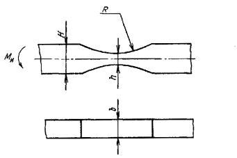
Fig. P2.7. The
shape and dimensions of the working part of the sample for
repeated bending tests:
|
h, mm
|
b, mm
|
H/h
|
R/h
|
|
2 - 10
|
(2 - 10)
|
1.5 - 2
|
≥ 5
|
9.7.12. The
equipment design shall be such that the fixing of the samples in the machine
grips, operations for setting it up to a given loading mode and installation of
the extensometer (resistance strain gauge) on the working part of the sample
can be carried out remotely using a manipulator.
Fig. P2.8. The
shape and dimensions of the working part of the sample for repeated torsion
tests:
|
d, mm
|
L, m
|
R, mm
|
|
3 - 10
|
3d
|
≥ d
|
9.7.13.
Extensometers and a dynamometric component of the machine shall be calibrated
at least 1 a year.
9.7.14. Test data
of exposed samples for low-cycle fatigue are processed in accordance with item 9.6.2.
9.7.15. Coefficient
φF (φFs) for given exposure conditions, is
determined as the ratio of the amplitudes of destructive deformations of the
samples of exposed eaF and unexposed ea
materials with the same number of cycles and are given in the form of φF
= f(ea)[φFs = f(ea)].
When determining the value of φFs, fatigue curves are used
which are the lower envelopes of the fatigue curves for different zones of the
welded joint or deposit welding, including transition zones.
10. METHODS FOR PROCESS
TESTS OF METALS
10.1. BENDING TEST METHOD
10.1.1. Process
bending tests at normal temperature, the shape and sizes of the samples shall
comply with the requirements of GOST 14019-80.
10.1.2. Results of
bending tests are assessed in accordance with the requirements of standards and
specifications for delivery.
10.2. PIPES. BENDING TEST METHODS
10.2.1. Bending
test methods for samples in the form of pipe sections, sample sizes, place for
cutting samples for testing, and assessment of results are determined in
accordance with the requirements of standards and technical specifications for
delivery.
10.3. PIPES. FLATTENING TEST METHOD
10.3.1. Flattening
test method, sample sizes, place for cutting samples for testing, and
assessment of tests are determined in accordance with the requirements of
standards and specifications for delivery.
11. WELDED JOINTS. METHODS
FOR DETERMINING MECHANICAL PROPERTIES
11.1.
Determination of the mechanical properties of a welded joint for static
tension, bending or flattening (for pipes with a wall thickness of up to s
= 12 mm – for impact bending), as well as static tension tests for the weld
metal, metal of various sections of the heat-affected zone and deposited metal
for all types welding, place of cutting, shape and size of samples, their
number, test conditions, and assessment of test results shall comply with the
requirements of
GOST 6996-66.
11.2. Static
bending tests of welded joints are carried out for butt welded joints:
shape and size of the
sample, place of sample cutting, requirements for sample preparation, and
bending test conditions are determined by GOST 6996-66; when the thickness of a
metal is more than 50 mm, the sample sizes are specified by special
specifications.
11.3. Flattening
tests are carried out on pipe sections, the sizes of which are determined by
GOST 6996-66; test conditions, assessment of test results are set according to
GOST 6996-66.
11.4. Impact
bending tests (for cut samples) of metal of various sections of a welded joint
and deposited metal are carried out in accordance with GOST 6996-66 on samples
of type IX or X, XI.
11.5. Static
bending tests of metal with deposit welding.
11.5.1. To test the
deposited corrosion-resistant coating for bending, control deposit weldings
made when validation of new materials are used.
11.5.2. Control
deposit welding is cut into two parts, one of which is used for the preparation
of bending samples without heat treatment, and the second is subjected to high
tempering before cutting samples according to production and process
documentation for the preparation of corresponding products with overlaying an
anti-corrosion coating.
11.5.3. Samples for
preparation for bending of deposited anti-corrosion coating.
11.5.3.1. Samples are
cut from the control deposit welding
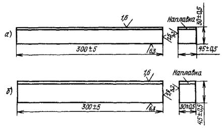
Fig. P2.9.
Types of samples:
a – type А1
and А2; b – type В1 and В2
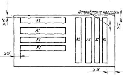
Fig. P2.10.
Sample cutting scheme:
A1 – with deposit welding
on the wide side with a longitudinal axis across the direction of deposit
welding; A2 – the same with a longitudinal axis along the direction of
deposit welding; В1 – sample with a deposit welding on the narrow side
with a longitudinal axis across the direction of deposit welding; В2 –
the same with a longitudinal axis along the direction of deposit welding of
four types, the shape and sizes of which shall comply with
Fig. P2.9 and P2.10.
|
направление наплавки
|
deposit welding direction
|
11.5.3.2. For certain
types of samples, the designations indicated in Fig. P2.10 are accepted.
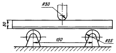
Fig. P2.11.
Scheme of testing samples of deposited metal
11.5.3.3. When
preparing samples, the following conditions shall be observed:
the surface of the
deposited coating is machined until the surface is leveled to ensure the
coating thickness within the established tolerances;
the direction of
machining shall coincide with a longitudinal axis of the sample;
the longitudinal edges
of samples shall be rounded with a radius of 0.5 mm.
11.5.4. Test
equipment.
Bending tests
of samples of the deposited anti-corrosion coating are carried out on testing
machines or presses of the appropriate capacity. In this case, the bending
radius of a punch and supports, as well as the distance between the supports,
shall correspond to Fig. P2.11, and the width of the punch and supports
shall exceed the width of the sample.
11.5.5. Testing.
11.5.5.1. The samples
are loaded smoothly with the punch movement speed of not more than 0.25 mm · s-1.
11.5.5.2. Bending
tests of samples of the deposited anti-corrosion coating are carried out with a
concentrated load in the middle of a span between the supports (Fig. P2.11)
before the occurrence of the first crack or to a given bend angle. Metal of
deposit welding, depending on the type of samples shall be located according to
Fig. P2.12.
11.5.6. Test
results assessment.
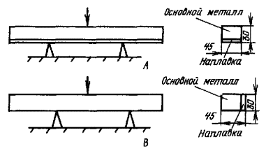
Fig. P2.12.
Sample arrangement when testing
|
наплавка
|
deposit welding
|
|
основной металл
|
base metal
|
11.5.6.1. When
testing for static bending, the outer surface and edges of the sample curved
part are examined without the use of magnifying means.
11.5.6.2. The bend
angle is measured in the unstressed state of the sample and is determined with
an error of no more than 2°.
11.5.6.3. When
bending tests before the occurrence of the first crack, the bending angle
obtained before the occurrence of the first crack in the stressed state is
determined.
11.5.6.4. Cracks
arising in the process of testing on the stretched side and on the edges of the
sample are not considered a rejection sign if their length does not exceed 20%
of the sample width and is not more than 5 mm, except for cracks arising in the
fusion zone of the anti-corrosion coating with the base metal.
When testing,
the place of formation of cracks or fracture is determined:
1) along the
seam;
2) along the
heat-affected zone;
3) along the
base metal.
11.5.6.5. Assessment
of test results is carried out depending on the requirements of the relevant
regulatory and technical documentation.
11.5.7. Test
protocol.
The test
protocol shall indicate:
1) grade and
batch of base metal;
2) grade and
batch of welding surfacing materials;
3) deposit
welding method;
4) type and
mode of heat treatment;
5) testing
method;
6) type and
size of sample;
7) labeling of
sample;
8) punch
mandrel diameter;
9) radius of
supports;
10) test
results.
APPENDIX 3
(recommended)
UNIFIED METHODS FOR DESIGN AND
EXPERIMENTAL DETERMINATION OF STRESSES, DEFORMATIONS, DISPLACEMENTS AND FORCES
Reference designations
s is a
thickness, mm
Rs is a mean shell radius,
mm
R is a current radius of thick-walled cylinder,
plate, ring, mm
R0 is a radius of the inner extreme point
of the ring, the inner radius of the branch pipe, mm
Rc is a radius of the
gravity center of cross section of the ring, the radius of the outer surface of
two-layer thick-walled cylinder, mm
Ra is an inner radius of a thick-walled
cylinder, mm
Rb is an outer radius of a
thick-walled cylinder, the radius of the total surface of a two-layer
thick-walled cylinder, mm
Rf is a fillet radius at the junction of
the branch pipe with the body, mm
Rp is an outer radius of the plate, the
radius of the outer extreme point of the ring, mm
Qi, Pi
are external forces distributed over the ring in the radial and vertical
direction, respectively, N/mm (kgf/mm)
M is a bending moment, N · mm (kgf · mm)
Mi is an external moment
distributed over the ring, N · mm/mm (kgf · mm/mm)
Nc is an uniformly distributed
force, referred to the gravity center of the cross section of the ring, N/mm
(kgf/mm)
Mc is a resultant moment,
referred to the gravity center of the cross section of the ring, N · mm (kgf ·
mm)
M0 is a concentrated bending moment, N · mm
(kgf · mm)
M1 is a bending moment applied to the
branch pipe in the meridional plane of the body, N · m (kgf · mm)
M2 is a bending moment applied to the
branch pipe in the cross-sectional plane of the body, N · mm (kgf · mm)
Mz, Mr, Mφ,
Mθ are axial, radial, meridional and ring bending moments,
respectively, N · mm/mm (kgf · mm/mm)
σz, σr,
σφ, φθ are axial, radial, meridional and ring stresses,
respectively, Pa (kgf/mm2)
Nz, Nφ, Nθ
are axial, meridional and ring forces, respectively, N/mm (kgf/mm)
H is a shear strain in the shell, acting in the
plane of a parallel circle, radial force in the plate, N/mm (kgf/mm)
θ is an angle of
rotation, rad
w is a radial
displacement of the shell, plate deflection, mm
u is a radial
displacement of the plate and ring, mm
ασ is a concentration
coefficient
m is a creep
indicator
z is a
distance from the edge along the axis of the cylindrical shell, for plates and
rings distance along the axis of ordinates, mm
l is a length
of a short cylindrical shell, mm
di, d is
a diameter of holes, mm
t is a pitch
of holes, mm
ni is a number
of holes with a diameter di
h is a height
of ring, mm
F is an effective cross-sectional area of ring,
mm2
Jx is a moment of inertia
of the ring cross section relative to the axis passing through the gravity center
of the ring cross section and perpendicular to the ring axis, mm4
F1 is a thickness ratio of abutting
components
φ is an angle, rad
φs is a
attenuation coefficient when stress calculation
φb is an
attenuation coefficient when bending
φc is a
attenuation coefficient when tension-compression
E is a modulus of longitudinal elasticity, Pa
(kgf/mm2)
μ is a Poisson ratio
α is a temperature
coefficient of linear expansion, 1/K (1/°C)
 - cylindrical
rigidity, N · mm (kgf · mm)
- cylindrical
rigidity, N · mm (kgf · mm)
 - coefficient
depending on material properties
- coefficient
depending on material properties
f is a
dimensionless function characterizing the law of variation of the edge moment
along the branch pipe generatrix
T is a temperature, K (°C)
p is a
pressure per surface unit, Pa (kgf/mm2)
pa is an
internal pressure per surface unit, Pa (kgf/mm2)
pb is an outer
pressure per surface unit, Pa (kgf/mm2)
P is a concentrated force, N (kgf)
1. BASIC PROVISIONS
1.1. This
Appendix to the Regulations contains recommended unified methods for design and
experimental determination of stresses, deformations, displacements and forces.
1.2. Along with
the described methods and formulas, it is allowed to use for the calculation
other calculation procedures and formulas that allow to obtain results with
greater accuracy.
2. CALCULATION OF
STRESSES, DISPLACEMENTS AND FORCES IN AXISYMMETRIC STRUCTURES OF THIN-WALLED
CLADDINGS, PLATES AND RINGS UNDER AXISYMMETRIC LOADING
2.1. RULE OF SIGNS
2.1.1. Positive
directions of forces and displacements (with the accepted reference direction
of the current coordinate along the meridian) for the cylindrical and spherical
shells, plate and ring are shown in Fig. P3.1.
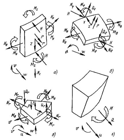
Fig. P3.1.
Positive directions of forces and displacements:
a is a
cylindrical shell; b is a spherical shell; c is a plate; d
is a ring
The signs
"±" in the formulas for stresses in the shells refer to the outer
"+" and inner "-" surfaces of the shells.
The signs
"±" in the formulas for stresses in the plates refer to the upper
"+" and lower "-" surfaces of the plate.
2.2. COMPONENTS OF ROTATION CLADDINGS UNDER EFFECTS
OF INTERNAL PRESSURE, TEMPERATURE LOADS, AND BOUNDARY FORCES
2.2.1. Cylindrical
thin-walled shell with constant thickness
Table P3.1
gives the formulas for calculating displacements, forces, and stresses in
cylindrical shell from uniform inner pressure and axial force, as well as from
hydrostatic pressure.
Table P3.2
gives the formulas for calculating displacements, forces, and stresses in
semi-infinite shell from an axisymmetric temperature field uneven along the
meridian and along the thickness.
Table P3.3
and P3.4 give the formulas for finding the displacements, forces, and
stresses, respectively, in semi-infinite (Table P3.3) and short (Table P3.4)
shells from edge shear forces and bending moments (no axial force) and given
edge displacements in short shells.
These formulas
are applicable if the radial displacements are small compared to the shell
thickness. When the ratio of s/Rs ≤ 0.05, error of
formulas is less than 5 %; at s/Rs ≤ 0.1 it is less
than 10 %. Shells can be considered as semi-infinite if their length is  Otherwise,
the formulas for the short shell shall be applied.
Otherwise,
the formulas for the short shell shall be applied.
2.2.2. Spherical
thin-walled shell with a constant thickness without a hole and with a hole at
the top (spherical segment).
Table P3.5
gives the formulas for calculating displacements, forces, and stresses in
spherical shell without a hole and with a hole at the top from a uniform inner
pressure and meridional tension force.
Table P3.6
gives the formulas for finding displacements, forces, and stresses in spherical
shell with no hole at the top from an axisymmetric temperature field uneven
along the meridian and along the thickness.
Table P3.7
gives the formulas for calculating displacements, forces, and stresses in
spherical shell with no hole at the top from the edge shear forces and bending
moments.
All formulas
are applicable for small radial displacements compared to the thickness and
under the following conditions for angles:
φ0,
φ1 – any (Table P3.5);
φ0
– any (Table P3.6);
φ*
≤ φ0 ≤ p - φ* (Tables P3.6, P3.7)
(at φ0 < φ*
=  , formulas
for spherical shell shall be applied).
, formulas
for spherical shell shall be applied).
Subject to the
specified conditions and ratio of s/Rs ≤ 0.05 the
error of the formulas is less than 5 %, at s/Rs ≤ 0.1
it is less than 10 %.
2.2.3. Elliptical
thin-walled shell with constant thickness (semi-ellipsoid).
Table P3.8
gives the formulas for calculating displacements, forces, and stresses in
elliptical shell from uniform inner pressure p and meridional tension
force Nφ = pa/2.
Table P3.1.
Formulas for displacements, forces, and stresses in a cylindrical thin-walled
shell. Load – inner pressure
|
Design
diagram
|
Considered
cross-section
|
Displacement,
force and tension
|
Note
|
|
Uniform inner pressure
p and axial force

|
Arbitrary, z = z
|
 
Mzp =0; Nθp
= pRφ;
Hzp = 0; Mθp
= 0;
 
|
a, b
are parameters
|
|
Hydrostatic pressure
linearly varying along the meridian,
p(z)
= az + b

|
Arbitrary, z = z
|
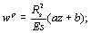
 Nzp = 0; Nzp = 0;
Mzp = 0; Nθp
= Rs(az + b);
Hzp = 0; Mθp
= 0;
σzp
= 0; 
|
-
|
Table P3.2. Formulas
for displacements, forces, and stresses in a semi-infinite cylindrical shell.
Load – axisymmetric temperature field
|
Design
diagram
|
Considered
cross-section
|
Displacement,
force and tension
|
Note
|
|
The temperature is
constant in thickness and in length of shell, T = T*
|
Arbitrary, z = z
|
wT = dRsT*;
 NzT = 0; NzT = 0;
MzT = 0; NθT
= 0;
HzT = 0; MθT
= 0;
σzT
= σθT = 0
|
-
|
|
The temperature is
constant in thickness and linearly varies in length, T(z) = az
+ b

|
Edge, z = 0
|
w0T = αRsb;
 Nz0T = 0; Nz0T = 0;
Mz0T = 0; Nθ0T = 0;
Hz0T = 0; Mθ0T
= 0;
σz0T
= σθ0T = 0
|
-
|
|
Arbitrary, z = z
|
wT = αRs(az
+ b);
 NzT = 0; NzT = 0;
MzT = 0; NθT
= 0;
HzT = 0; MθT
= 0;
σzT
= σθT = 0
|
-
|
|
The temperature is
constant in thickness and varies in length along a square parabola, T(z)
= az2 + bz + c
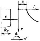
|
Edge, z = 0
|

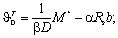 NTφ0 = 0; NTφ0 = 0;
Mz0T = 0; 
Hz0T = 0; Mθ0T = 0;
σz0 = 0; 
|
M* = -2DαRsa;

f1 = e-xcosx;
f2 = e-xsinx;
f3 = f1
– f2;
f4 = f1
+ f2;
x = βz
|
|
Arbitrary, z = z
|
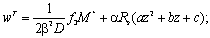
 NzT = 0; NzT = 0;
MzT = (1-f4)M*;

HzT = -2βf2M*;
MθT = μMzT;
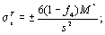 
|
|
Away from the edge, 
|
wT = αRs(az2
+ bz + c);
 NzT = 0; NzT = 0;
MzT = M*;
NθT = 0;
HzT = 0; MθT
= μMzT;
 σθT
=μσzT σθT
=μσzT
|
|
|
The temperature
linearly varies in thickness; the temperature mean in thickness is zero
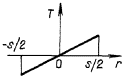
|
Edge, z = 0
|

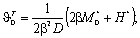 Nφ0T = 0; Nφ0T = 0;
Mz0T = 0; 
Hz0T = 0; Mθ0T = (1 – μ)M0*;
σz0T
= 0; 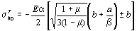
|
|
|
The temperature
difference between the outer and inner surfaces of ∆T either does not
vary in length (∆T = b), either varies in length linearly (∆T
= az + b)
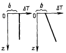
|
Arbitrary, z = z
|
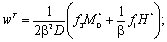
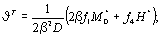 NzT = 0; NzT = 0;
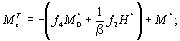 
HzT = -(2βf2M0*
+ f3H*) + H*; MθT
= μMzT + (1 – μ)M*;
 
|
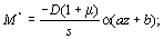
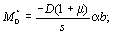
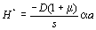
|
|
Away from the edge,
|
wT = 0;
 NzT = 0; NzT = 0;
MzT = M*;
NθT = 0;
HzT = H*;
MθT = M*;

|
-
|
Table P3.3. Formulas
for displacements, forces, and stresses in an axisymmetric cylindrical
semi-infinite shell with a constant thickness.
Load
– axisymmetric edge forces
|
Design
diagram
|
Considered
cross-section
|
Displacement,
force and tension
|
Note
|
|
Forces M0
and H0 at the edge, z = 0
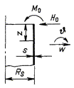
|
Edge, z = 0
|
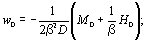
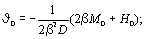 Nz0 = 0 Nz0 = 0
Mz0 = M0;

Hz0 = H0;
Mθ0 = μM0;
 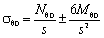
|

f1 = e-xcosx;
f2 = e-xsinx;
f3 = f1
– f2;
f4 = f1
+ f2;
x = βz
|
|
Arbitrary, z = z
|
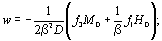
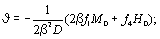 Nz = 0 Nz = 0
 
Hz = 2βf2M0
+ f3H0; Mθ = μMz;
 
|
|
Table P3.4. Formulas
for displacements, forces, and stresses in an axisymmetric cylindrical short
shell with a constant thickness.
Load
– axisymmetric edge displacements and forces
|
Design
diagram
|
Considered
cross-section
|
Displacement,
force and tension
|
Note
|
|
At the edge, z
= 0, known forces M0, H0 and
displacements w0, 
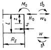
|
Arbitrary, z = z
|
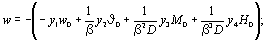
 Nz = 0; Nz = 0;
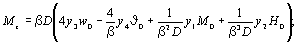 
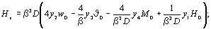 Mθ = μMz; Mθ = μMz;

|
y1 = cosxchx;
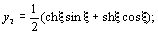

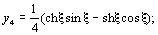
x = βz; 
|
|
At the edge, z
= 0 and z = l, given forces M0, H0,
M1, H1
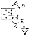
|
Edges, z = 0, z
= l
|
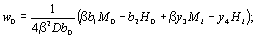
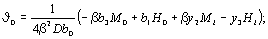
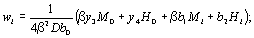
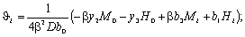
|
b0 = y32
– y2y4;
b1 = y1y3
– y22;
y2 = y2y3
– y1y4;
y3 = y1y2
+ 4y3y4;
Calculated at x = βl
|
|
Arbitrary, z = z
|
w, θ, Mz,
Hz calculated by the formulas of this table, which
substitute the specified effort M0, H0,
as well as displacements w0,  ,
calculated by the formulas of the same table ,
calculated by the formulas of the same table
|
|
Table P3.5. Formulas
for displacements, forces, and stresses in an axisymmetric spherical shell with
constant thickness without a hole and with a hole at the top. Load – inner
pressure
|
Design
diagram
|
Considered
cross-section
|
Displacement,
force and tension
|
Note
|
|
Uniform inner pressure
and meridional tension force
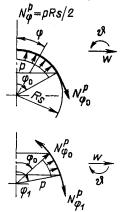
|
Arbitrary, φ = φ
|
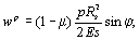
 
Mφp = 0; 
Hφp = 0; Mθp
= 0;

|
-
|
Table P3.6. Formulas
for displacements, forces, and stresses in an axisymmetric spherical shell with
constant thickness with no hole at the top.
Load
– axisymmetric temperature field
|
Design
diagram
|
Considered
cross-section
|
Displacement,
force and tension
|
Note
|
|
The temperature is
constant in thickness and along meridian, T = T*
|
Arbitrary, φ = φ
|
wT =αRsT*sin
φ;
 NTφ = 0; NTφ = 0;
MTφ = 0; NTθ
= 0;
HTφ = 0; MTθ
= 0;
σTφ
= σTθ = 0
|
-
|
|
The temperature is
constant in thickness and varies linearly along the rotation axis, T(x)
= ax + b; x = Rscos φ
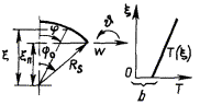
|
Arbitrary, φ = φ
|
wT =αRssin
φ(aRscos φ + b);
 NTφ = 0; NTφ = 0;
MTφ = 0; NTθ
= 0;
HTφ = 0; MTθ
= 0;
σTφ
= σTθ = 0
|
-
|
|
The temperature
linearly varies in thickness; the temperature mean in thickness is zero, the
temperature difference between the outer and inner surfaces does not change
along the meridian, ∆T = a
|
Edge, φ = φ0
|
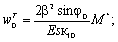
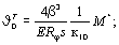 Nφ0T = 0; Nφ0T = 0;
Mφ0T = 0; 
Hφ0T = 0; Mθ0T = (1 – μ)M*;
 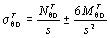
|
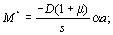
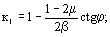
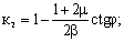
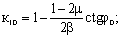
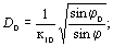
f1 = e-xcosx;
f2 = e-xsinx;
x = β(φ0 –
φ)
|
|
Arbitrary, φ = φ
|
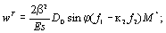
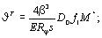 NφT = 0; NφT = 0;
 
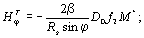 MθT = μMφT + (1 + μ)M*; MθT = μMφT + (1 + μ)M*;
 
|
|
Away from the edge, 
|
wT = 0;
NφT = 0;
MφT = M*;
NθT = 0;
HφT = 0; MθT
= M*;
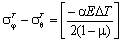
|
Table P3.7.
Formulas for displacements, forces, and stresses in an axisymmetric spherical
shell with constant thickness with no hole at the top. Load – axisymmetric edge
forces
|
Design
diagram
|
Considered
cross-section
|
Displacement,
force and tension
|
Note
|
|
At the edge, φ = φ0,
given forces M0, H0
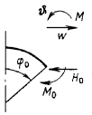
|
Edge, φ = φ0
|
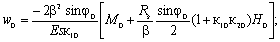
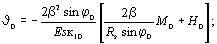
Mφ0 = M0;
Hφ0 = H0
|
 
|
Nφ = -cosφHφ;
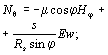

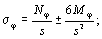

|
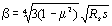
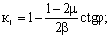
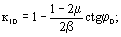
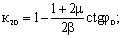
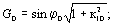
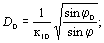
f1 = e-xcosx;
f2 = e-xsinx;
f3 = e-xcos(x
+ γ);
f4 = e-xsin(x
+ γ);
γ = arctg(-к10);
x = β(φ0 –
φ)
|
|
Arbitrary, φ = φ
|
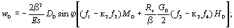
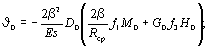
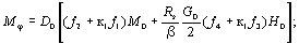
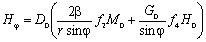
|
|
The same for
hemisphere, φ0 = p/2
|
Edge, φ = p/2
|
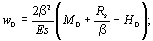
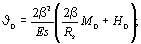
Mφ0 = M0;
Hφ0 = H0
|
Table P3.8. Formulas
for displacements, forces, and stresses in an axisymmetric elliptical shell
with a constant thickness.
Load
– inner pressure and tension force
|
Design
diagram
|
Considered
cross-section
|
Displacement,
force and tension
|
Note
|
|
Uniform inner pressure
and meridional tension force
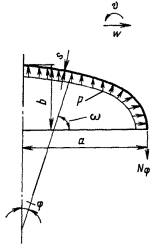
|
Edge, φ = p/2
|
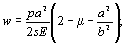


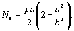 
Mφ = Mθ
= Hφ = 0; 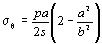
|
Shell curvature radii,
 R2
= a R2
= a
|
|
Arbitrary
|
 
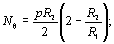 
Mφ = Mθ
= Hφ = 0;
|


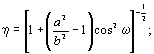
ω = p/2 - φ
|
|
Pole,
φ = 0
|
 
Mφ = Mθ
= Hφ = 0;
|
R1 = R2
= a2/b
|
Table P3.9. Formulas
for displacements, forces, and stresses in an axisymmetric elliptical shell
with a constant thickness.
Load
– axisymmetric edge forces
|
Design
diagram
|
Considered
cross-section
|
Displacement,
force and tension
|
Note
|
|
At the edge, φ = p/2,
given forces M0 and H0
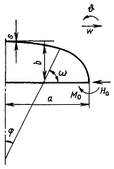
|
Edge, φ = p/2
|
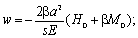
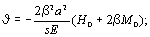
Nφ = 0; Nθ
= -2βa(H0 + βM0);
Mφ = M0;
Mθ = μM0;

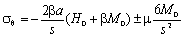
|

|
|
Arbitrary
|
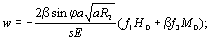
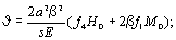
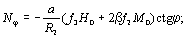
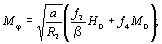

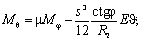
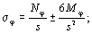

|
f1 = e-1cosx;
R2 – see in
Table P3.8;
f2 = e-xsinx;
f3 = f1
– f2;
f4 = f1
+ f2;
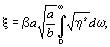
R1, R2,
η, ω – see in Table P3.8
|
Table P3.10. Formulas
for displacements, forces and stresses in round solid plates with constant
thickness, hinge-supported along the edge. Load – uniform pressure and
axisymmetric shear and bending forces
|
Design
diagram
|
Displacement,
force and tension
|
|
in an
arbitrary cross-section
|
in the center
|
on the
edge
|
|
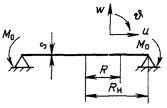
|
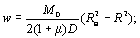


Mr = Mθ
= M0;
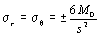
|


u = 0;
Mr = Mθ
= M0;
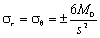
|
w = 0;


Mr = Mθ
= M0;
|
|
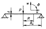
|
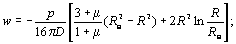
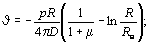
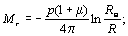
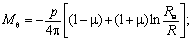
 
|
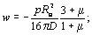
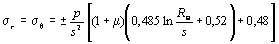
|
w = 0;
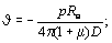


σr =
0;
|
|
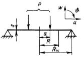
|
R < a
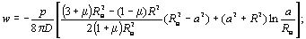
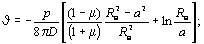
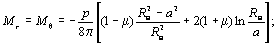
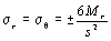
|
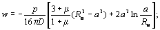
u = 0;

|
-
|
|
|
R > a
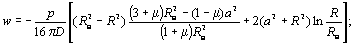
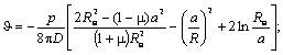
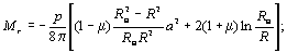
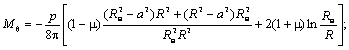
|
-
|
w = 0;
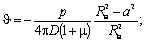
Mr = 0;
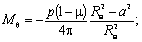
σr =
0;
|
|
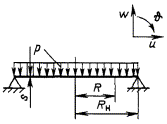
|
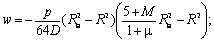
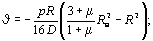
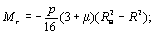
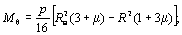
|
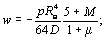
u = 0;
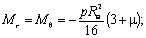

|
w = 0;

Mr = 0;
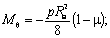

|
|
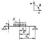
|
R < a
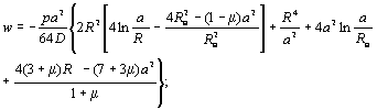
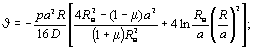
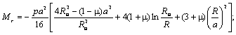
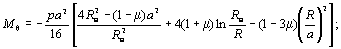
 
|
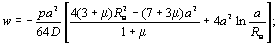

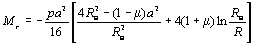
|
-
|
|
R > a
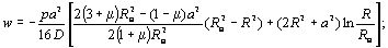
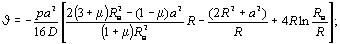

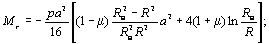
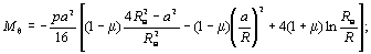
|
|
w = 0;
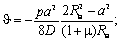

Mr = 0;
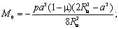
σr
= 0;
|
Table P3.9
gives the formulas for determining displacements, forces, and stresses in
elliptical shell from the edge shear forces and bending moments.
2.3. ROUND PLATES UNDER EFFECTS OF POWER AND
TEMPERATURE LOADS
Table P3.10
gives the formulas for calculating displacements, forces, and stresses in round
solid plates, hinge-supported along the edge, from uniformly distributed, shear
and bending loads for an arbitrary cross-section and characteristic places
(edge and center).
Table P3.11
gives the formulas for determining displacements, forces, and stresses in ring
plates, hinge-supported along the external circuit, from uniformly distributed,
shear and bending loads for an arbitrary cross-section and on the edges.
Table P3.12
gives the formulas for finding displacements, forces, and stresses in round
solid and ring plates from an axisymmetric tension load.
Table P3.13
gives the formulas for calculating displacements, forces, and stresses in round
solid and ring plates from temperature loads (the temperature varies along the
radius and thickness of the plate).
Formulas are
applicable if the plates are thin, i.e. the ratio of thickness to outer radius
does not exceed 0.2, and if the deflections are small compared with the plate
thickness.
When
calculating perforated plates, in the formulas for displacements of w, θ
in Table P3.10, P3.11 instead of D use D1
= Dφb, for displacements of u in Table P3.12
add φc in the denominator, for stresses (Table P3.10 -
P3.12) add φs in the denominator.
In the case of
a uniform perforation over the entire surface of the plate (establishing of the
holes is triangular or square), the attenuation coefficient is determined by
the following dependencies:
a)
when calculating bending displacements
φb
= 1.18(t – d)/t;
b)
when calculating tension (compression) displacements of the plate in the radial
direction
φс = (t – d)/t;
c)
when calculating stresses
φs =(t – d)/t.
Table P3.11. Formulas for
displacements, forces and stresses in ring plates with constant thickness,
hinge-supported along the external circuit. Load – uniform pressure and
axisymmetric shear and bending forces
|
Design
diagram
|
Displacement,
force and tension
|
|
in an
arbitrary cross-section
|
on the
inner edge (R = R0)
|
on the
outer edge (R = Ro)
|
|
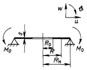
|

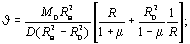

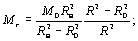

|
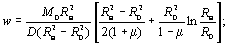
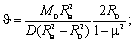

Mr = 0;

σr =
0;
|
w = 0;
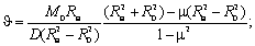
Mr = Mθ;
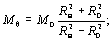
|
|
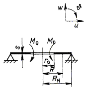
|
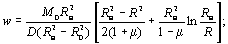
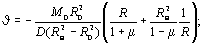
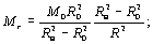
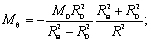
|
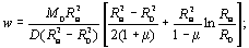
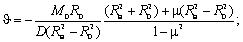
Mr = M0;
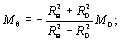
|
w = 0;
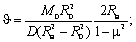
Mr = 0;
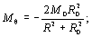
σr =
0;
|
|
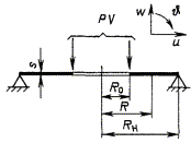
|
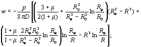
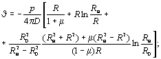
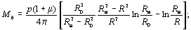
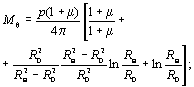
|
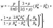

Mr = 0;
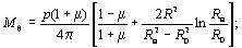
|
w = 0;
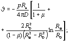
Mr = 0;
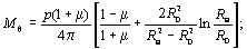
σr =
0;
|
|
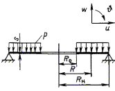
|
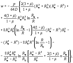
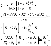
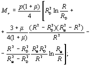
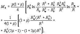
|
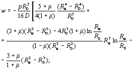
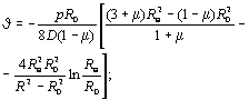
Mr = 0;
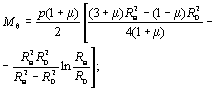
σr =
0;
|
w = 0;
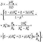
Mr = 0;
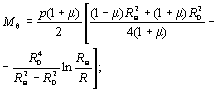
σr =
0;
|
Table P3.12. Formulas
for displacements, forces, and stresses in round solid and ring plates with
constant thickness.
Load
– axisymmetric tension forces
|
Design
diagram
|
Displacement,
force and tension
|
|
in an
arbitrary cross-section
|
in the center
|
on the
edge
|
|
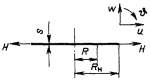
|

Hr = Hθ
= H;
σr
= σθ = H/s
|
-
|

Hr = Hθ
= H;
σr
= σθ = H/s
|
|
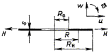
|
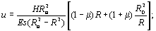
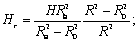 
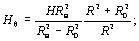 
|

Hr = 0;
 
|
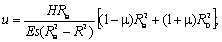
Hr = H;
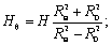
|
|
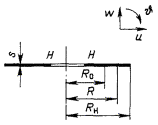
|
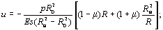
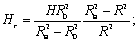
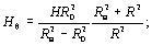
|
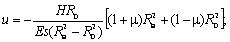
Hr = H;


|
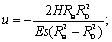
Hr = 0; σr
= 0;

|
Table P3.13. Formulas
for displacements, forces, and stresses in round solid and ring plates. Load –
temperature field
|
Design
diagram
|
Displacement,
force and tension
|
|
in an
arbitrary cross-section
|
in the center
|
on the
edge
|
|
Solid round plate with
radial temperature variation t(R)
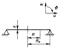
|
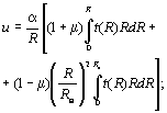

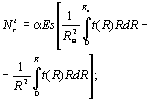
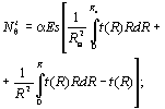
Mtr = Mtθ
= 0;
 
|
u = 0;
w = 0;
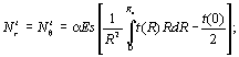
Mtr = Mtθ
= 0;

|
u = 0;
w = 0;

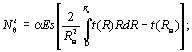
Mtr = Mtθ
= Ntr = 0;
|
|
Solid round plate with
temperature variation in thickness under an arbitrary law
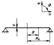
|
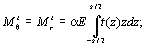
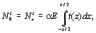
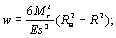
 
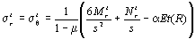
|


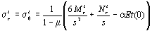
|
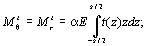
w
= 0;

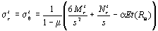
|
|
Solid round plate with
temperature variation in thickness under a linear law
|
σtr
= σtθ = 0
|
σtr
= σtθ = 0
|
σtr
= σtθ = 0
|
|
Displacements
and forces are calculated using the formulas for a solid round plate with
temperature variation in thickness under an arbitrary law
|
|
Ring round plate with
radial temperature variation t(R)
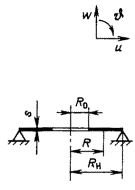
|
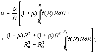

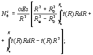
Mtr = Mtθ
= 0;
σtr
= Ntr/s;
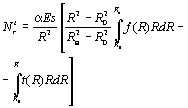
|
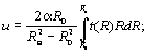

Ntr = 0;
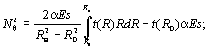
Mtr = Mtθ
= 0;
σtr
= 0;
σtθ
= Ntθ/s
|
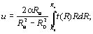
Ntr = 0;
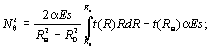
Mtr = Mtθ
= 0;
σtr
= 0;
σtθ
= Ntθ/s
|
|
Ring round plate with
temperature variation in thickness under an arbitrary law t(z)
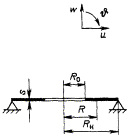
|
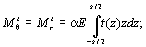
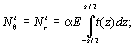
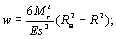

|
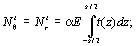
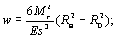


|
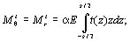


w = 0;
|
|
Ring round plate with
temperature variation in thickness under a linear law
|
σtr
= σtθ = 0
|
σtr
= σtθ = 0
|
σtr
= σtθ = 0
|
|
Displacements
and forces are calculated using the formulas for a ring plate with variation
in thickness under an arbitrary law
|
Table P3.14. Formulas
for determining displacements and stresses in the ring from power loads
|
Design
diagram
|
Considered
cross-section
|
Displacement
|
Stress
|
Note
|
|
Ring having an
arbitrary shape in its cross-section and loaded with distributed loads
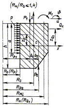
|
Passing through the
gravity center
|

|

|

 
|
|
Arbitrary
|
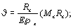

|
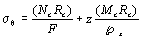
|
|
The design diagram is
the same 
|
Passing through the
gravity center
|
|
|


|
|
Arbitrary
|
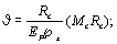
|
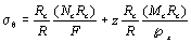
|
Table P3.15. Formulas
for determining displacements and stresses in the ring from temperature loads
|
Design
diagram.
Type of
loads
|
Coordinate
|
Displacement
|
Stress
|
|
Ring having an
arbitrary shape in its cross-section and an arbitrary temperature
distribution t(x, z)
Rand/R0
≤ 1.6; h/R0 ≤ 0.6
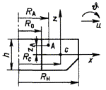
|
Arbitrary point A
|
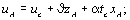


|
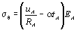
|
|
The design diagram is
the same Rand/R0 ≤ 3; h/R0
≤ 0.6
|
|
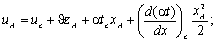


|
|
Table P3.16. Formulas
for determining forces and stresses in the simplest composite structures due to
the action of internal pressure
|
Design
diagram
|
Considered
cross-section
|
Boundary
force
|
Stress
|
Note
|
|
Connection of a
cylindrical shell with a spherical segment
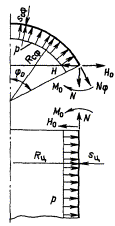
|
Cylinder joint with a
spherical segment
|
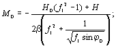

where 
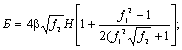
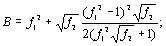
f2 = f1sinφ0
|
Spherical
segment (φ = φ0):

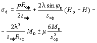
Cylinder (x
= 0):
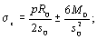
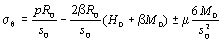
|
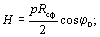


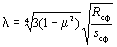
|
|
Connection of a
cylindrical shell with a semi-ellipsoid:
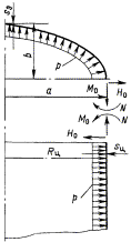
|
Cylinder joint with a
semi-ellipsoid
|
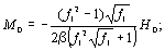
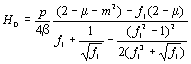
At f1
= 1 (se = sc)
M0 = 0;

|
Elliptical shell:
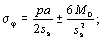
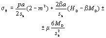
Cylinder:
|
f1 = se/ss;
a = Rc
m =a/b
|
|
Joint of cylindrical
shells of different thickness
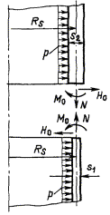
|
Joint of cylinders
|
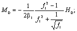
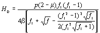
|
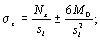
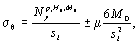
 – for
both cylinders; – for
both cylinders;
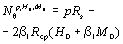 – for
cylinder with a thickness of s1; – for
cylinder with a thickness of s1;
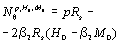 – for
cylinder with a thickness of s2 – for
cylinder with a thickness of s2
|

f1 = se/ss;


|
|
Connection of a
cylindrical shell with a plate
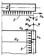
|
Joint of components
|
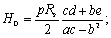
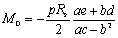
|
Cylinder:
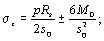
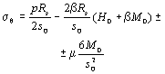
|
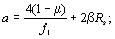
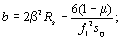
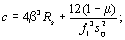
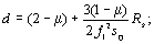


|
|
Connection of a
cylindrical shell with a ring
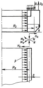
|
Joint of components
|


|
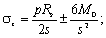

|
For 
(see
Section 2.4)
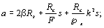
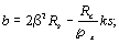
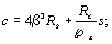
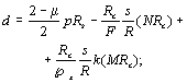
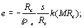

(NRc)
and (MRc) are determined according to Section 2.4
|
If the holes
have unequal diameter or are located unevenly, then when determining the
attenuation coefficients, the most weakened plate diameter or a series of holes
located near the diameter are considered. Accordingly we have
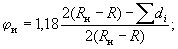
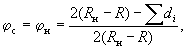
where di
are diameters of holes located in the row under consideration. In this case, it
is assumed that uniform attenuation is maintained in the plate.
2.4. RING PARTS UNDER EFFECTS OF POWER AND
TEMPERATURE LOADS
Table P3.14
gives the formulas for displacements and stresses under the effect of power
load on the ring.
Internal
forces acting in the cross-section of the ring (in relation to the design
scheme in Table P3.14),
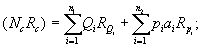
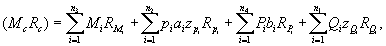
where (NcRc)
is a force perpendicular to the cross-section of the ring;  are
radii of stress application; (McRc) is a bending
moment relative to the axis x;
are
radii of stress application; (McRc) is a bending
moment relative to the axis x;  are coordinates of
points of force application piai and Qi;
bi is a force action arm Pi (for other
designations see Table P3.14).
are coordinates of
points of force application piai and Qi;
bi is a force action arm Pi (for other
designations see Table P3.14).
The transverse
forces Q1 and the pressure p directed from the axis of
the ring, and the moments from the forces causing clockwise rotation of the
cross-section, are assumed as positive directions.
Table P3.15
gives the formulas for displacements and stresses with an arbitrary temperature
distribution T(x, z) in the cross-section of the ring when
the modulus of elasticity and the coefficient of linear expansion in the
cross-section of the ring are variable: E(x, z), α(x,
z).
2.5. COMPLEX STRUCTURES
Table P3.16
gives examples of composite structures, consisting of two components and loaded
with uniform inner pressure. Thin-walled shells, plates and rings are
considered as the components of structures.
Formulas for determining
the forces and stresses are given for the junction of the components in
question. In order to find the forces and stresses in an arbitrary
cross-section of a component, one shall use the corresponding expressions for
this component, summing up algebraically their values from loading by inner
pressure and boundary forces H0 and moments M0
obtained for this composite structure, and for the spherical segment the
difference (H0 - H), with due regard to the presence
of thrust force, shall be assumed as H0. Formulas are given
provided that the elastic moduli of the materials of the mating components of
structures are the same.
3. CALCULATION OF
STRESSES AND DISPLACEMENTS IN AXISYMMETRIC THICK-WALLED COMPONENTS OF
STRUCTURES
3.1. The
calculation of stresses and displacements in the hollow cylinder from a uniform
pressure and temperature differences in the cross-sections, at a distance 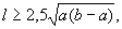 from the
edges, is given in Tables P3.17, P3.18.
from the
edges, is given in Tables P3.17, P3.18.
3.2. The
formulas for calculating displacements and stresses in a hollow cylinder made
of a homogeneous material are given in Table P3.17.
3.3. The
formulas for calculating displacements and stresses in a double-layered
cylinder are given in Table P3.18. These formulas take into account the
compatibility of work of the cylinder layers in the axial and radial directions
(there is no slippage of layers and no possibility of the formation of gaps
between the layers).
4. CALCULATION OF LOCAL
STRESSES IN COMPONENTS OF STRUCTURES
In the zone of
sudden changes in geometry (holes, fillets, undercuts, etc.): there is a local
increase in stress. In the case of elastic deformations, the maximum stresses σmax
in this area are determined as the product of the nominal stress σnom
and so-called theoretical concentration coefficient ασ:
σmax
= ασσnom.
The
concentration coefficients ασ given in this section are obtained by
experiment or calculation. Each figure or table shows the
nominal stresses in relation to which the concentration coefficients are
determined.
Table P3.17. Formulas
for displacements and stresses in a cylinder made of a homogeneous material
|
Design
diagram
|
Radius
|
Displacement
|
Stress
|
Note
|
|
Pressure
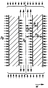
|
Arbitrary
|
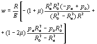
|
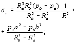
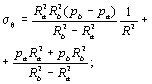
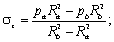
|
-
|
|
R = Ra
|
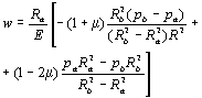
|
σr =
-pa;
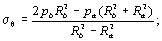
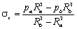
|
-
|
|
R = Rb
|
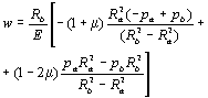
|
σr =
-pb;
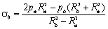
|
-
|
|
Temperature loads T
= T(R)
|
Arbitrary
|
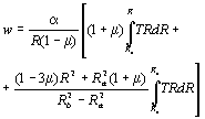
|
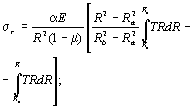
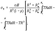
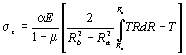
|
-
|
|
R = Ra
|
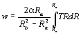
|
σr =
0;
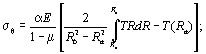
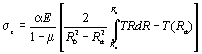
|
-
|
|
R = Rb
|
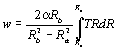
|
σr
= 0;
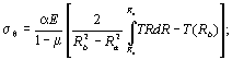
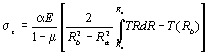
|
-
|
Table P3.18. Formulas
for displacements and stresses in a double-layer cylinder
|
Design
diagram
|
Radius
|
Displacement
|
Stress
|
Note
|
|
Internal pressure
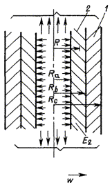
|
Arbitrary
|
Layer 1
|
|
|
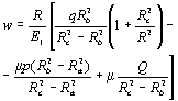
|
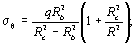
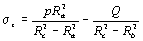
|
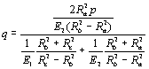
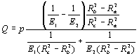
|
|
R = Rb
|
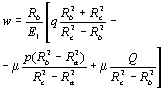
|

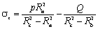
|
-
|
|
R = Rc
|
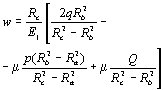
|

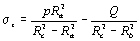
|
-
|
|
Arbitrary
|
Layer 2
|
|
|
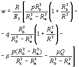
|
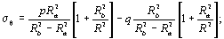
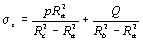
|
|
|
R = Rb
|
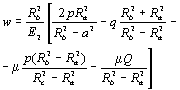
|
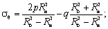
|
-
|
|
R = Ra
|
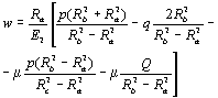
|
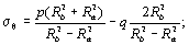
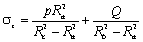
|
-
|
|
Temperature loads
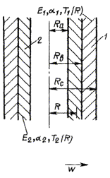
|
Arbitrary
|
Layer 1
|
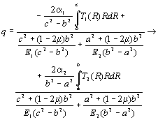
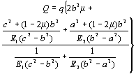
|
|
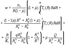
|
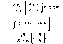

|
|
R = Rb
|
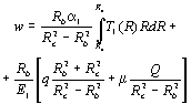
|
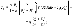
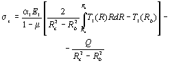
|
-
|
|
R = Rc
|
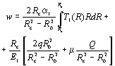
|
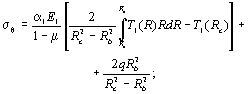

|
-
|
|
Arbitrary
|
Layer 2
|
|
|
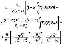
|
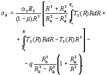
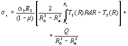
|
-
|
|
R = Rb
|
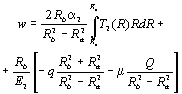
|
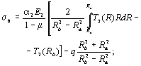
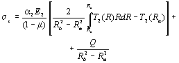
|
-
|
|
R = Ra
|
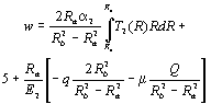
|
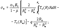
|
-
|
This section
contains formulas and graphs for determining the coefficients ασ
under elastic deformations from the effect of force loads, taken from
well-known published works. They are presented for the following types of
concentrators:
single holes in plates
(Fig. P3.2 - P3.10);
a group of circular
holes in plates (Fig. P3.11 - P3.16);
supported holes and
branch pipes (Fig. P3.17 - P3.26);
junction zones of the
components of structures (Fig. P3.27 - P3.33);
surface and subsurface
defects (Fig. P3.34 - P3.37);
some types of welded joints
(Fig. P3.38).
The figures
given in the section use the following conventional symbols:
R is a radius of a fillet, hole, mm
D is a diameter of a hole, cylinder, mm
H is a thickness of a plate, shell, mm
S is a width of a plate, bridge between holes, mm
L is an intercenter distance, hole distance from
plate edge, mm
P is a tension force, N (kgf)
M is a bending moment, N · m (kgf · m)
p is an inner
pressure, Pa (kgf/mm2)
A, B, C are the most dangerous
points
v is a Poisson
ratio
β is an angle between
the direction of force and the line of centers of holes, rad
γ is an angle of
inclination of a fillet, rad
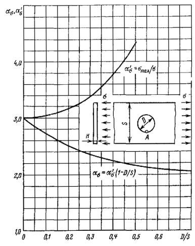
Fig. P3.2.
Coefficients ασ and α'σ for point A of a stretched
plate of finite width with a centrally located circular hole
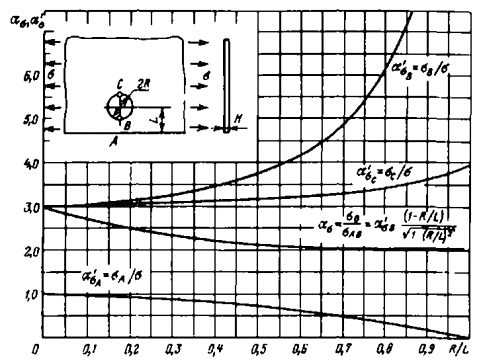
Fig. P3.3.
Coefficients ασ for point B and α'σ for
points A, B and C of a stretched semi-infinite plate with
a circular hole located at the edge
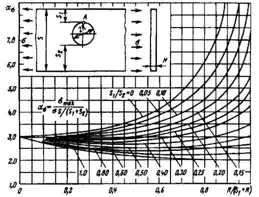
Fig. P3.4.
Coefficients ασ for point A of a stretched plate of finite
width with a non-central circular hole
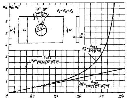
Fig. P3.5.
Coefficients ασ (σnom calculated at point A), α"σ
(σnom calculated at point C) and α'σ for
point A of a thin bending bar with a central circular hole
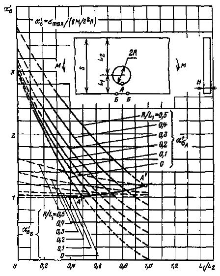
Fig. P3.6.
Coefficients α'σ for points A and B of a thin
bending bar with non-central circular hole on line A'A' 
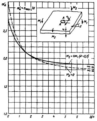
Fig. P3.7.
Coefficients α'σ for point A of an unlimited plate
with a circular hole at clean (M2 = 0) and cylindrical (M2
= vM1) bends
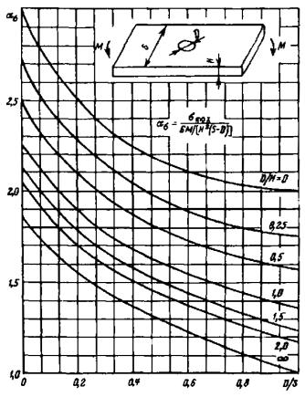
Fig. P3.8.
Coefficients ασ at transverse bending of a plate with finite width
with a central circular hole
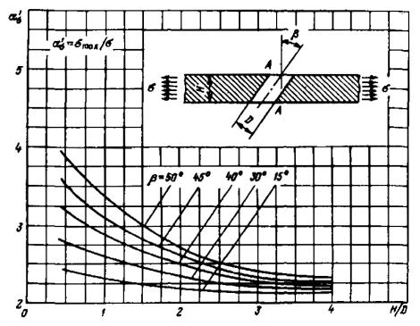
Fig. P3.9. Coefficients
α'σ for point A of an unlimited plate with an oblique
hole at biaxial tension
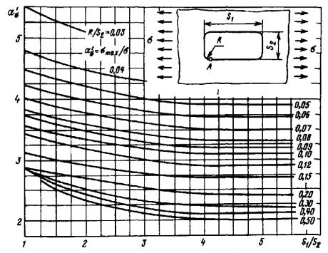
Fig. P3.10.
Coefficients α'σ for point A of an unlimited stretched
plate with a rectangular hole with rounded corners
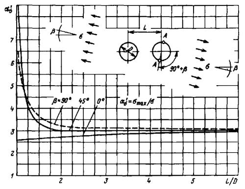
Fig. P3.11.
Coefficients α'σ for point A of an infinite plate with
two equal circular holes when stretched at an angle to the line of the centers
of holes
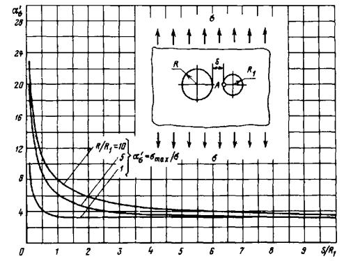
Fig. P3.12.
Coefficients α'σ for point A of an infinite plate with
two unequal circular holes when stretched perpendicular to the line of the centers
of holes
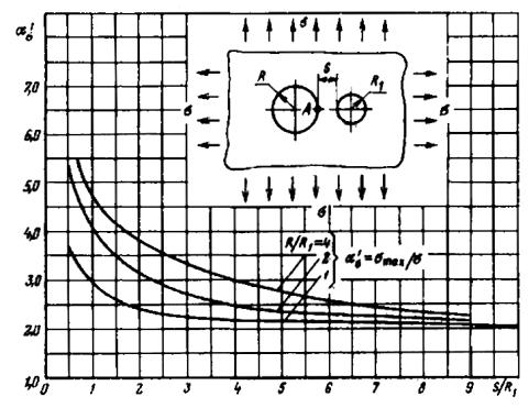
Fig. P3.13.
Coefficients α'σ for point A of an infinite plate with
an uneven circular holes at biaxial tension
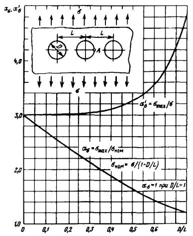
Fig. P3.14.
Coefficients ασ and α'σ for point A of an
unlimited plate with an infinite row of circular holes when stretched perpendicular
to the line of the centers of holes
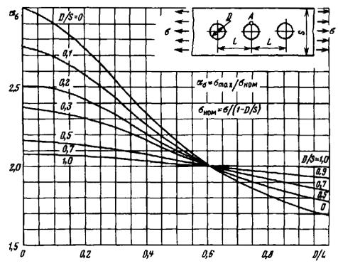
Fig. P3.15.
Coefficients ασ for point A of a stretched plate of finite
width with an infinite row of circular holes
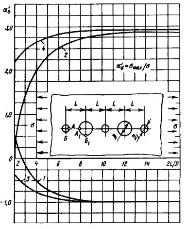
Fig. P3.16.
Coefficients α'σ for stretched plate with periodically
located circular holes of different diameters at D/D1
= 4:
1 – for point A; 2
– for point B; 3 – for point A1; 4 – for
point B1

Fig. P3.17.
Coefficients α'σ for point A of stretched plate with a
supported circular hole at
D/H = 5
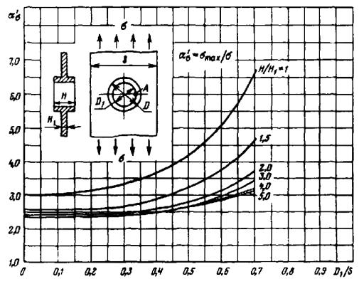
Fig. P3.18.
Coefficients α'σ for point A of stretched plate with a
reinforced hole at D1/D = 0.7 and D/H =
5
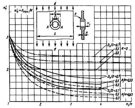
Fig. P3.19.
Coefficients α'σ for point A of a stretched plate with
a supported circular hole and fillets from support to plate at S/D
= 4 and D/H = 5
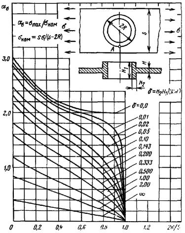
Fig. P3.20.
Coefficients ασ for point A of a stretched plate of finite
width with a central circular hole supported with a thin ring
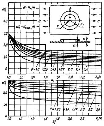
Fig. P3.21.
Coefficients α'σ for stretched unlimited plate with one-sided
supported holes:
a – for point A
on the junction line; b – for point B on the inner surface of a
hole
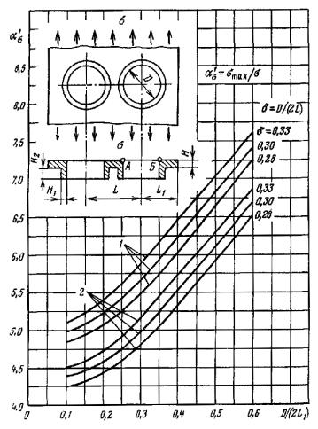
Fig. P3.22.
Coefficients α'σ for stretched plate with two adjacent
one-side supported holes (Н1 = Н, Н2
= 2Н):
1 – for point A; 2
– for point B
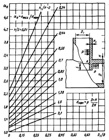
Fig. P3.23.
Loading by inner pressure of a cylindrical vessel with a missed branch pipe
(ασ for point A)
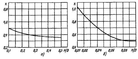
Fig. P3.24.
Correction coefficient K for determining α'σ = Kασ
in supported holes of vessel with H/D ≥ 0.01 for ασ,
found according to Fig. P3.23:
a – for H/D
from 0.1 to 0.5; b – for H/D from 0.01 to 0.1
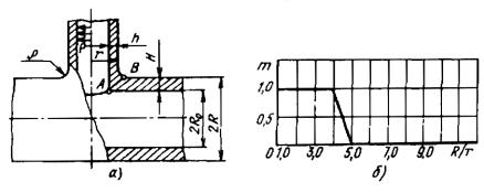
Fig. P3.25.
Determination of stress concentration coefficients at points A and B
of a tee connection loaded with inner pressure:
a is a tee
connection diagram; b is a correction coefficient graph m
For tee
connectors equal in strength, it is allowed to use the formulas
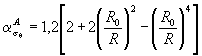
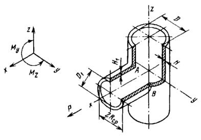
Fig. P3.26.
Branch pipe loading with moments and tension force (formulas for determining ασ
for each type of load are given below)
|
Load
type
|
Formula
for determining ασ
|
Nominal
stress σnom
|
Point of
maximum stresses
|
Limit of
applicability of formula
|
|
My
|
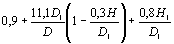
|

|
A
|

|
|
Mz
|
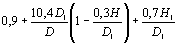
|

|
C
|

|
|
P
|
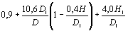
|

|
C
|

|
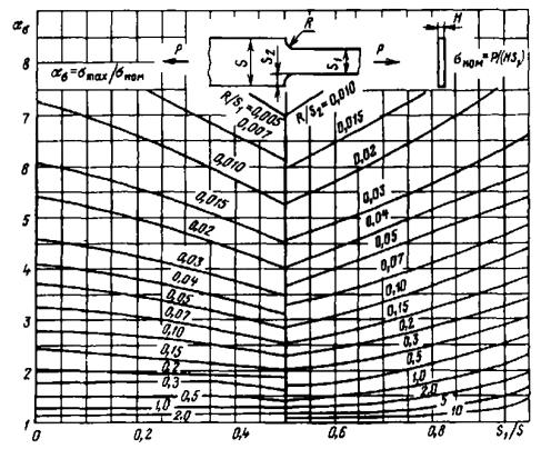
Fig. P3.27.
Coefficients ασ for a stretched flat stepped rod with fillets
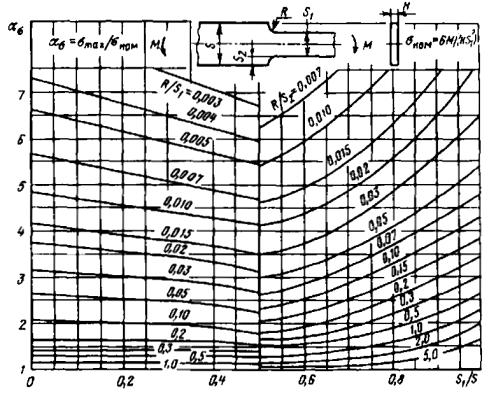
Fig. P3.28.
Coefficients ασ for a bending flat stepped bar with fillets
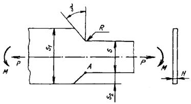
Fig. P3.29.
Stepped flat bar with inclined fillets loaded with axial force and bending
moment. Formulas for determining concentration coefficients for point A
are given below
|
Force
factor
|
Nominal
stress σnom
|
Formula
for determining ασ
|
Formula
for determining K
|
|
|
P
|

|
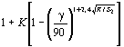
|
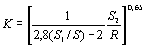
|
|
|
M
|

|
|
|
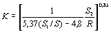
|
|

Fig. P3.30.
Coefficient ασ for point A of bending angle component
(recommended to apply at Н1/Н = 1)
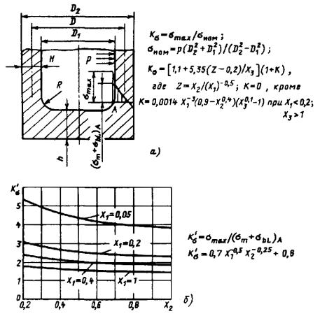
Fig. P3.31.
Stress concentration coefficients for point А Kσ(a) and K'σ(δ)
of a cylindrical vessel with a flat head:
X1 = R/H 0.05 ≤ X1
≤ 1
X2 = D/(20H) 0.2 ≤ X2
≤ 1
X3 = h/Н 1 ≤ X3
≤ 4
|
где
|
where
|
|
кроме
|
except
|
|
при
|
at
|
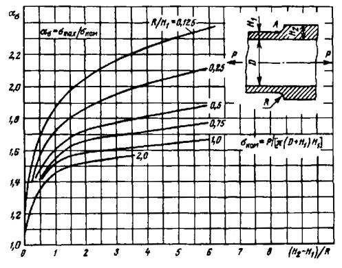
Fig. P3.32.
Coefficients ασ for point A of stretched pipe with a stepped
change in wall thickness and fillets
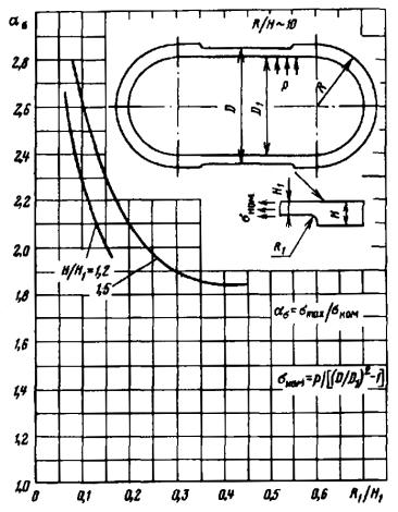
Fig. P3.33.
Coefficient ασ for loading with inner pressure the vessel with a
stepped change in wall thickness and fillets

Fig. P3.34.
Coefficient α'σ for stretched unlimited plate with small
spherical depressions on both surfaces
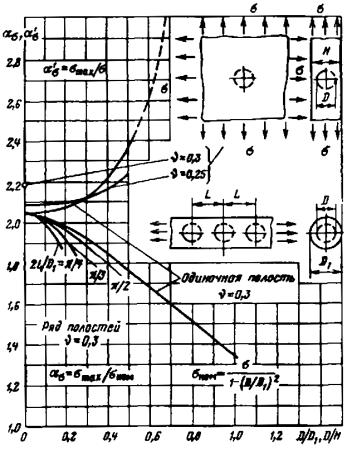
Fig. P3.35.
Coefficients ασ and α'σ for stretched plate and
cylinder with a central spherical cavity
|
одиночная полость
|
single cavity
|
|
ряд полостей
|
row of cavities
|
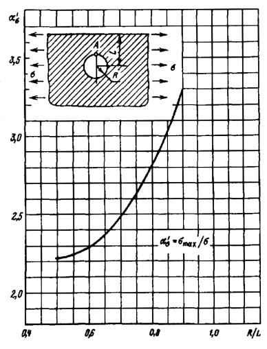
Fig. P3.36.
Concentration coefficients α'σ for point A when
biaxially tension of a semi-infinite body with a spherical cavity near the
surface (v = 0.25)
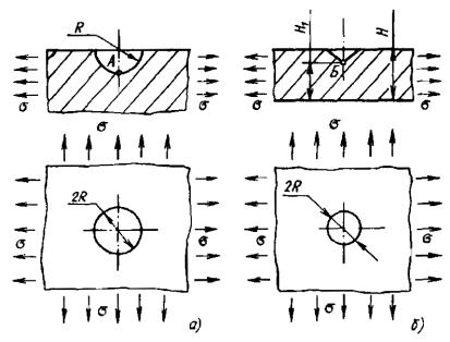
Fig. P3.37.
Some types of surface defects in the stretched components:
a is a
semi-infinite body with a hemispherical depression; b is a plate with
hyperbolic depression (values of concentration coefficients ασ for
points A and B are given below)
|
Load
case
|
Nominal
stress σnom
|
Value ασ
|
|
Fig. P3.37,
a
|
σ
|
2.23 (v
= 0.25)
|
|
Fig. P3.37,
b
|
3.8
|
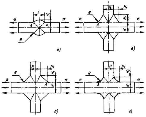
Fig. P3.38.
Welded joints and workload application diagram:
a is a butt
joint; b is a cross joint with a seam formed by the hypotenuse of a
multifaceted triangle; c is a cross joint with a seam in a form of an
isosceles triangle; d is a cross joint with wave-shaped seams (formulas
for ασ are given below)
|
Type
of welded joint
|
Nominal
stress σnom
|
Formula
for determining ασ for point A
|
|
Fig. P3.38,
a
|
σ
|

|
|
Fig. P3.38,
b
|
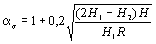
|
|
Fig. P3.38,
c
|
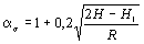
|
|
Fig. P3.38,
d
|
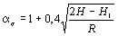
|
5.
EXPERIMENTAL DETERMINATION OF STRESS AND DISPLACEMENT DEFORMATIONS
5.1. GENERAL
5.1.1.
Conventional symbols used in this Section:
α is a scale of
geometric similarity
l is a linear
size, mm
β is a scale of force
similarity
P is an external load force, N (kgf)
E is a modulus of elasticity of material, Pa
(kgf/mm2)
δ is a scale of
displacement similarity
u is a linear
displacement
η is a scale of
similarity of moments
M is a moment of external load, Nm (kgf · mm)
σ is a stress, Pa
(kgf/mm2)
σmL is
a local membrane stresses, Pa (kgf/mm2)
σbL is
a local bending stresses, Pa (kgf/mm2)
σm is
a general membrane stresses, Pa (kgf/mm2)
σb is
a general bending stresses, Pa (kgf/mm2)
σaF is
a local stress amplitude with due regard to concentration, Pa (kgf/mm2)
σnom is a
nominal stresses, Pa (kgf/mm2)
p is a
pressure per surface unit, Pa (kgf/mm2)
Q is an internal force in cross-section, N (kgf)
m is an
internal moment in cross-section, N·m (kgf · mm)
ε is a relative
deformation, RU
ε1, ε2
is a principal relative deformations, RU
γxy is
a relative shear or angular deformation, RU
G is a shear modulus, Pa (kgf/mm2)
 is an arithmetic mean of
observations in the absence of load (zero value)
is an arithmetic mean of
observations in the absence of load (zero value)
 is an observation
value
is an observation
value
 is an arithmetic mean of
observations
is an arithmetic mean of
observations
n is a number
of repeated observations
n1 is a number
of abnormal observations
S* is a general standard deviation
Sn is a standard deviation
of instrument errors
ψ is a maximum value of
deviation for a given sample size according to n observations and an
accepted level of significance of 0.05. Determined according to GOST 8.207-76
D is an outer surface diameter, mm
H is a wall thickness, mm
C1 is a wall thickness tolerance, mm
φ0 is an
angle between deformation axes ε1 and ε0, rad
Ri is a strain-sensitivity of an instrument
Rr is a strain-sensitivity of a resistance
strain gauge
N is a number of repeated loads
N1 is a number of abnormal deformation
values
ασ is a stress
concentration coefficient.
Indices:
i is a
sequence number of repeated observation
j is a
sequence number of loading step
k is a
measurement point number
k is a
resistance strain gauge number
p is a real
value
f – full size, outer
m – model
b – bend; v –
inner
5.1.2. This
Section contains recommendations for experimental determination of stresses,
deformations and displacements.
5.1.3.
Deformations, stresses and displacements are experimentally determined on
full-size parts and components of structures or on their models. Experimental
studies on models can be carried out at all stages of the design of objects.
Experimental studies on full-size objects can be carried out at the
manufacturing stages, during factory and start-up tests, and operation.
5.1.4. Stresses,
deformations and displacements are experimentally determined using strain
measurement and photoelastic method. Other experimental methods (fragile
coatings, grade grids, moire fringes) are also allowed. When selecting a
method, it shall be shown that its capabilities match the measurement problems
and conditions.
5.2. OBJECTIVES, OBJECTS AND CONDITIONS OF
CONDUCTING EXPERIMENTAL STUDIES
5.2.1.
Experimental studies of stresses, deformations and displacements of parts and
components of structures shall be carried out in cases when it is impossible to
determine with the necessary accuracy the characteristics of the
stress-deformed state of the structure. In this case, the assessment of the
object strength shall be based on information obtained from the experiment.
5.2.2.
Experimental studies shall provide information on the stress-deformed state of
the structure, which is necessary to test the structure for strength in
accordance with the standards of strength.
5.2.3. The object
of experimental study may be a full-size part, a structure or a corresponding
model made of full-size or another material, including polymeric one.
5.2.4. Selection
of the object of study is determined by the operation conditions of the
full-size part or structure. It is necessary to distinguish the following main
cases of operation of full-size structures with possible combinations of
existing power and temperature loads:
a) the largest
deformations do not exceed the yield limit;
b) the deformation
exceeds the yield limit.
5.2.5. For case
a), the experimental study of the stresses of deformations and displacements
can be carried out on a full-size structure or its model, made of any
materials, but satisfying the similarity conditions in elastic
("elastic" model).
5.2.6. In case b)
the study shall be carried out on a full-size structure or model made of the
same materials as the full-size structure ("full-size" model), with
loads corresponding to the operating ones, i.e. creating the same relative
deformations according to distributions and values. It is allowed to use models
made of other materials, but providing similarity conditions in the elastic and
plastic ("elastic plastic" model).
5.2.7. Types of
loads, their limiting numerical values and possible combinations for full-size
structure are set by the designer based on the operating parameters, operating
modes and conditions of the surveillance testing of the designed equipment, and
are specified in the task for the experimental study.
5.2.8. In the
study of individual parts of full-size structures or corresponding models, it
is necessary to reproduce the boundary conditions, which can be determined on
the grounds of a calculation or an experimental study of the entire structure.
It is allowed to conduct tests at loads exceeding those determined in the
calculation or from the experiment.
Boundary
conditions can be reproduced by creating the corresponding efforts or
displacements on the border, as well as by using additional components adjacent
to the investigated part and affecting it in a given way.
5.2.9.
Measurements of deformations and displacements shall be carried out in strictly
established, controlled and recorded conditions under the action of force and
temperature loads in accordance with the specified modes.
5.3. ELASTIC MODELS AND TERMS OF THEIR LOADING
5.3.1. Models and
loads applied to them shall meet the relevant modeling conditions ensuring the
possibility of transition from deformations, stresses, and displacements in the
model to deformations, stresses, and displacements in full size.
5.3.2. The model
shall be made in full compliance with the geometric and force similarity to
full-size one. The places of application of loads in the model shall correspond
to the places of their application in full size, and the values of all applied
loads in the model and in full size shall be proportional with the same
proportionality coefficient for all loads. Permissible deviations of the
geometric dimensions and external force factors in the model and in full size
shall be consistent in accordance with the requirements of the geometric and
force similarity. Deviation from complete similarity, which does not lead to a
change in the stress-deformed state in the studied zones, is allowed. At the
same time, any deviations from the full geometrical and force similarity, inter
alia the replacement of a three-dimensional model with a flat one, shall be
justified on case by case basis. Both theoretical and experimental data can be
used to substantiate.
5.3.3. The
materials and model manufacturing technology used shall ensure that all sizes
and shape features, that affect the stress state of the structure under study,
are in place.
5.3.4. If the
full-size structure is made of materials with different elastic moduli, then
its elastic model shall be made of materials having the same ratios of elastic
moduli.
5.3.5. In studies
of thermoelastic stresses with the use of heating or cooling, it is necessary
to make models of materials with the same ratios of products of the temperature
coefficient of linear expansion and modulus of elasticity, which have the
materials of corresponding parts of the full-size structure.
5.3.6. Values of
the greatest loads on elastic models made of a material different from the
material of full size are selected so that the deformations in the model do not
exceed the limit of proportionality, and the strength conditions of the model
are also provided.
In the case of
a model of low-modulus materials, such as plastics, the greatest loads shall be
limited to such values that when they are applied, there is no distortion of
geometric shape of the model, affecting the resulting stresses and
displacements.
5.3.7. In the
"elastic" models with a linear dependence between loads and
displacements, stress and displacement from the simultaneous action of all
loads can be obtained on the grounds of the principle of superposition, i.e.
corresponding addition at each considered point of results obtained from
individual loads. The principle of superposition is not preserved when there is
a non-linear dependence between loads and displacements, for example, when full
take-up of clearances in the loading process, when presence of extensive
contact zones that affect stresses in the studied areas. In this case, the
study shall be performed with the simultaneous action of all loads.
5.3.8. If there
are composite contacting parts in the "elastic" model, where friction
forces can act and clearances and contact conditions can change, it is
necessary to implement corresponding dependences in the model. In this case,
the connection of parts with tension, ensuring the absence of mutual
displacement of the position of the contacting surfaces, can be considered as
monolithic. In contact zones, it is sufficient to correctly make resultant
forces only if the stresses are determined in places remote from these zones.
5.3.9. The results
of measurements of deformations and displacements obtained for linear problems
(linear dependence of stresses and displacements on load under various load
cases) shall be recalculated according to similarity criteria for full-size
structure for the values of design loads. In the case of non-linear problems,
the results obtained shall be referred to the loads of the full-size structure
corresponding to those for which the measurements were carried out.
5.4. CONDITIONS FOR ELASTIC MODELING AND
RECALCULATING RESULTS OF THE STUDY FOR A FULL-SIZE STRUCTURE
5.4.1. The model
shall be made geometrically similar to the full size with respect to the scale
of geometric similarity
α = lf/lm.
5.4.2. Values of
loads applied to the model are determined by values of loads in full size with
respect for the scale of force similarity
β = Pf/Pm.
5.4.3. In the
general case of modeling, it is necessary that the deformation of full size and
of model are the same. This shall be done if the clearances taken-up during
loading lead to a change in the stress distribution in the zones in question or
if large displacements are simulated. At the same time, the scales of geometric
and force similarity are related by the dependence
β = α2Ef/Em,
and the scale of linear
dimensions is equal to the scale of displacements
δ = uf/um.
5.4.4. In cases
where the displacements in the model are sufficiently small and do not lead to
a violation of the geometric similarity of the model and full size or to the
nonlinear dependence of stresses on the load, the scales of geometric α and
force β similarity can be assigned independently.
5.4.5. If the
conditions of item 5.4.4 are met if the models have clearances and
process tolerances taken-up during the loading process, then they shall be
performed not on the scale of geometric similarity, but on a scale of
displacements

which may be different
from the scale of geometric similarity α.
5.4.6. Moments of
the loads applied to the model are calculated according to the scale
η = Mf/Mm,
which is not independent
and shall be determined by the formula
η = αβ.
5.4.7.
Recalculation of displacements, stresses and internal force factors from model
to full size is carried out according to the formulas given in Table P3.19,
which correspond to the case of independence of the scales α and β and
inequality of the scales α and δ, the formulas are also valid in the case of
item 5.4.3.
5.5. STRAIN MEASUREMENT
5.5.1. Strain
measurement is one of the main experimental methods for studying the stress and
strain state of structures when studying the behavior of full-size objects
during the period of commissioning and operational work, as well as studying
the stress state of structures in laboratory conditions on models at the design
stage.
This method is
used in a wide range of deformations, temperatures and fluxes of ionizing
radiation when affecting the objects of static, quasistatic and dynamic loads.
Table P3.19. Formulas
for recalculating experimental data from model to full size
|
Type
of external load
|
Recalculated
value
|
|
Tension σ
|
Inner
moment m
|
External
force Q
|
Linear
displacement u
|
|
Pressure p
|

|

|

|

|
|
Bending moment M
|

|
mf = ηmm
|

|

|
|
Focused force P
|

|
mf = αβmm
|
Qf = βQm
|

|
|
Linear displacement u
|

|

|

|
uf = δum
|
5.5.2. Types of
resistance strain gages shall be selected subject to the goals and conditions
of the experiment.
For studies,
you shall use resistance strain gauges manufactured in series in domestic (or
foreign) enterprises, passed calibration control and having a certificate
containing their metrological characteristics. When using non-standard
resistance strain gauges, the metrological characteristics of the resistance
strain gauges and procedures by which they are determined shall be reported.
5.5.3. When strain
measurement in conditions of elevated temperatures, self-compensated resistance
strain gages and circuit compensation methods or methods of amending according
to the metrological characteristics of the used resistance strain gages are
used.
5.5.4. The means
of protecting the resistance strain gauges from aggressive media and mechanical
damage shall not affect the metrological characteristics of the resistance
strain gauges and distort the stress state of the component under study.
5.5.5. All
instruments used to measure deformations and temperatures, before each test or
series of tests, shall undergo metrological calibration using standard
instrumentation. Instruments shall be calibrated at least 2 times a year.
5.5.6. When
conducting complex tests, it is advisable to automate the process of measuring
and registering data, to use computers to process the results of experiments.
5.5.7. The
registration of observations when an object is tested at each step of loading
(mode) is repeated at least 3 times. (Practically the multiplicity of repeated
observations is 3-15.)
5.5.8. The results
of observations for mathematical processing are presented in the form of a
sequence of numbers as a function of time (registration on digital printers or
punching apparatuses) or in the form of tables (compiled by the experimenter).
5.5.9. To
determine the actual value of readings of each resistance strain gauge at each
step of loading  , ordering of
the sample of observations is carried out, namely:
, ordering of
the sample of observations is carried out, namely:
calculate the mean value

check the significance
of each of the n observations according to condition

and in the case of
non-compliance of the inequality, recognize this observation as abnormal and
exclude it from the sample under consideration;
calculate as the
arithmetic mean of significant observations of the sample
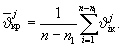
5.5.10. With a
single observation, a single reading (observation) of the instrument is taken
as a valid measurement result. The error of the result is estimated by the
results of the calibration of strain-gauge transducers and devices
(strain-gauge measurement system as a whole) or by the errors indicated in the
certificate data.
5.5.11.
Deformations are determined by actual observations
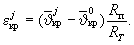
If it is
possible to repeat the loading conditions of the object of study, the values of
relative deformations are determined for each repeated loading, and then the
ordering of the sample of relative deformations is performed by N
repeated loading
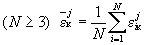
and their significance
is checked

Actual value
of the deformations is determined by the formula
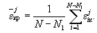
5.5.12. With
known dependencies of deformations on loads, the actual value of deformations
shall be determined by the least squares method using the alignment technique.
Table P3.20. Determination
of the principal deformations ε1 and ε2 and their
directions according to the measured relative deformations
|
Type
of stress state and location of the resistance strain gauges
|
Relative
deformations measured by a resistance strain gauge
|
Determination
of ε1, ε2, ηxy and of main
directions
|
|
Resistance
strain gages are located in known directions of main deformations.
|
|
Linear stress state
(direction ε1)

|
ε0
|
ε1 = ε0;
ε2 = -με0
|
|
Flat stress state
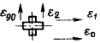
|
ε0, ε90
ε0 ≥ ε90
|
ε1 = ε0;
ε2 = ε90
|
|
Directions
of main deformations are unknown
|
|
Flat stress state (angles
between axis and axes of the resistance strain gauges 0, 45° and 90°)
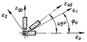
|
ε0, ε45,
ε90
|
γxy = 2ε45
– (ε0 + ε90)
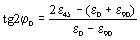
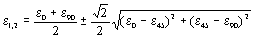
|
|
Flat stress state
(angles between axis and axes of the resistance strain gauges 0, 60° and
120°)
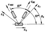
|
ε0, ε60,
ε120
|
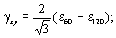
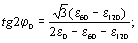
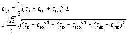
|
5.5.13. The main
deformations ε1, ε2 and their directions are determined
in accordance with Table P3.20 according to actual values of
deformations.
5.5.14. The main
stresses σ1 and σ2 are determined from the main
deformations, σ1 and σ2 are determined from the main
deformations ε1 and ε2 at the measurement points of the
part (model) by the formulas:
for flat stress state
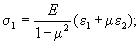
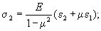
for uniaxial stress
state
σ1
= Eε1.
Maximum shear
stresses are determined by the formula
τxy
= Gγxy.
5.5.15.
Recalculation of stresses from the model to full size is carried out by the
formulas given in Section 5.4.
5.5.16. The
structure strength for the stresses obtained experimentally is estimated in
accordance with Section 4 hereof.
5.5.17. The results
of strain measurement are presented by categories and groups of stress
categories, regulated by the assessment of strength of the structures under
study (Table P3.21).
5.6. PHOTOELASTIC METHOD
5.6.1. The
photoelastic method is used to determine the fields of deformations and
stresses in parts and structures under the static force loads and temperature
fields. It is used primarily in laboratory and bench tests for the study of
areas with high stress gradients.
5.6.2. Studies by
the photoelastic method are performed on models of transparent optically sensitive
materials or with the use of coatings applied to the surface under study made
of optically sensitive materials.
5.6.3. Network
polymers, such as hardened epoxy resins, are commonly used as optically
sensitive materials for models and coatings.
Optically
sensitive material shall have sufficient transparency and optical sensitivity
to deformation, optical isotropy in the undeformed state and stability of the
optical and mechanical properties over time. Mechanical properties of the
material for the model shall ensure that the similarity criteria of the model
and the full-size sample are met, and mechanical properties of the material for
the coatings shall ensure the possibility of joint deformation of coating and
surface of the part under study while maintaining the linear dependence of the
optical effect on deformations throughout the entire range of deformations of
surface of the part under study.
Table P3.21. Examples
of stress categories construction
|
Object
of the study
|
Stress
categories
|
Formula
|
|
Body, pipeline, branch
pipe, etc.
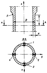
|
Local membrane*
σmL (at  ) )
|
0.5(σkf
+ σkv)
|
|
Compensation of
tension or compression* σcm
|
|
|
General bending*
 from
bending moment My from
bending moment My
|
0.5(σ1f
+ σ1v – σ3f – σ3v)
|
|
General bending*
 from
bending moment Mx from
bending moment Mx
|
0.5(σ2f
+ σ2v – σ4f – σ4v)
|
|
General bending*
σb from bending moment 
|

|
|
Local bending*
σbL
|
0.5(σkf
– σkv)
|
* Determined
in cross-section A-A.
5.6.4. Elastic
stresses in a three-dimensional structure from the action of static force loads
are determined using a three-dimensional model investigated by the method of
deformation "freezing". In this case, stresses can be determined both
on the surface and inside the structure under study.
5.6.5. Elastic
stresses on the outer surface of the structure under the action of several
alternately applied static force loads are determined on the
"elastic" model (see item 5.2.5 of this Appendix) using
coatings made of optically sensitive material. It is also possible to carry out
study on models using the method of deformation "freezing". In this
case, the required number of models is equal to the number of separately
considered loads.
5.6.6. Elastic
plastic stresses and deformations on the outer surface of a structure under the
action of a static force load are determined on a full-size structure or its
"full-size" model (see item 5.2.6 of this Appendix) using
coatings made of optically sensitive material.
5.6.7. Elastic
stresses in a structure made of materials with different linear expansion
coefficients are determined from the action of a uniform temperature field on a
three-dimensional "frozen" model composed of components with
previously "frozen" deformations corresponding to free temperature
expansions taken with the opposite sign.
5.6.8.
Thermoelastic stresses from the action of static and quasistatic (slowly
varying in time) temperature fields are determined using a three-dimensional
"frozen" model composed of components with previously
"frozen" deformations corresponding to free temperature expansions
taken with the opposite sign.
APPENDIX 4
(recommended)
CALCULATION OF COMPONENTS OF STRUCTURES
FOR PROGRESSIVE FORM CHANGE
1. GENERAL
1.1. This
Appendix to the Regulations contains the basic provisions and the method of
calculation for progressive form change.
1.2. This
material is recommended to be used when carrying out a checking calculation for
progressive form change according to Section 5.10 hereof.
1.3. Along with
the given methods and formulas, it is allowed to use for the calculation other
methods and formulas that, inter alia, allow to obtain results with greater
accuracy.
1.4. When
calculating the progressive form change, changes in the shape and size of the
structure resulting from both the process of accumulation of irreversible
plastic deformations continuously increasing with an increase in the number of
cycles, and irradiation growth, are determined.
1.5. Conditions
for the occurrence of progressive form change of components of structures are
determined according to the theory of adaptability of elastic plastic bodies
with repeated loads and experimental data.
1.6. Calculation
for progressive form change is carried out for the cases specified in Section 5.10
hereof. The rules of calculation do not apply to threaded connections, keys,
dowels, etc.
1.7. The
calculation is carried out for normal and abnormal operation, with due regard
to all the design loads specified in item 5.1.3 hereof.
1.8. Conditions
for occurrence and development of progressive form change are influenced by the
mechanical loads and temperature, as well as by the nature of their change (by
volume of structure and in time), geometric features of the part (sizes, fixing
method, etc.), temperature and time dependence of mechanical characteristics of
the material, and irradiation growth.
1.9. A necessary
condition for the onset of progressive form change is the non-simultaneity of
maximum stress at different points of the part. Extreme in this sense, external
influences are cyclically repetitive moving mechanical loads and
"moving" (quasistationary relative to the moving coordinate system)
temperature fields.
Temperature
fields of this type, inter alia, can occur in the walls of vessels with cyclic
changes in the coolant level, with a rapid change in the coolant temperature,
with a rapid change in heat generation in the pipes, inside of which there are
structures with a sufficiently large heat capacity.
2. DEFINITIONS. RATED
STRESSES
2.1. Here, the
cycle of stress changes in all modes under normal and abnormal operation is
called the working cycle; and mechanical, thermal and other loads are its
parameters.
2.2. The cycle
of stress changes, which corresponds to the beginning of a progressive form
change, i.e. is the boundary between progressive form change and adaptability,
is called the limit.
Progressive form change
means the process of accumulation of one-sided plastic irreversible
deformations (displacements), non-simultaneous in terms of volume of the
component of structure, small in each cycle of changes in stresses and
temperatures.
Adaptability of the structure
means the termination of cyclic plastic deformation after a certain number of
first cycles, mainly due to the formation of a favorable residual stress field.
2.3. During the
first calculation stage (Section 5 hereof), conventional stresses in the
working cycle σi(e) from mechanical loads
and uneven heating of the structure are used (calculated under the assumption
of ideal elasticity of material). The corresponding reduced stresses are
calculated according to the theory of the greatest shear stresses.
2.4. Conditional
elastic stresses in the limit cycle are proportional to the conditional elastic
stresses of the operating cycle, i.e. ratio of the indicated stresses n
is the same for all points of the structure for all modes constituting the
cycle.
2.5. Conditional
elastic stresses in the operating cycle are calculated separately for
steady-state modes and for a number of time moments of transients. Modes and
times within individual modes for which stresses σi(e)
are calculated shall be selected so that at the end, in each point of the
structure, it is possible to find the minimum (during the cycle) difference
between limit σs (which are selected different depending on
the operating modes of operating cycle in accordance with Section 3 of
this Appendix) and reduced conditional elastic stresses.
2.6. Conditional
elastic stresses in the operating cycle σi(e)
for bodies and internal parts of reactors, steam generators and vessels are
obtained by summing the general or local membrane stresses, general and local
bending stresses, and general temperature stresses (including stresses due to
temperature variations across the wall thickness).
2.7. Conditional
elastic stresses in the operating cycle σi(e)
for pipelines are obtained by summing general or local membrane stresses,
general and local bending stresses, general temperature stresses (including
stresses due to temperature gradients across the wall thickness), and
compensation stresses (membrane, torsion and bending).
3. LIMIT STRESSES
3.1. For
transients, limit stress σs is assumed to be equal to yield
limit of the material RTp0.2 divided by
the coefficient:
σs
= RTp0.2/n0.2,
where n0.2
= 1.5; nmt =1.5.
The value of RTp0.2
is assumed in accordance with items 3.7 and 3.8 hereof at the
structure point temperature which is in effect at the considered time of the transient.
3.2. For
steady-state operation modes, the limit stress is assumed equal to
σs
= min{RTp0.2/n0.2; RTmt/nmt},
where n0.2
= 1.5; nmt = 1.5.
The values of RTp0.2
and RTmt are assumed in accordance with items 3.7
and 3.8 hereof at the design temperature of metal in a steady-state
mode, with due regard to the possible reduction of their values during neutron
exposure.
4. ADDITIONAL
CONVENTIONAL SYMBOLS
σs is
a limit stress, MPa (kgf/mm2)
σi(e)
are conditional elastic stress components in the operating cycle, MPa (kgf/mm2)
n is a ratio
of conditional elastic stresses in the limit cycle to the corresponding
stresses of the operating cycle
σφ(e),
σθ(e), σr(e)
are meridional, ring and radial components of the conditional normal elastic
stress in the operating cycle, MPa (kgf/mm2)
ρφ, ρθ,
ρr are residual stress components, MPa (kgf/mm2)
h is a half
thickness of the shell (plate), mm
z is a
coordinate measured from the middle surface of the shell (plate) along the
normal to this surface, mm
t is time
(from the beginning of the cycle), h
∆ε is a cumulative
deformation per cycle, %
∆l is an
irreversible l length change, mm.
5. SEQUENCE OF
CALCULATION FOR PROGRESSIVE FORM CHANGE IN THE ABSENCE OF IRRADIATION GROWTH
5.1. Reduced
conventional elastic stresses in the operating cycle calculated in Section 3
of the this Appendix are compared with the limit stresses σs.
If the reduced elastic stresses at all points of the structure do not exceed σs,
then the structure works elastically in all cycles (starting from the first).
In this case, the progressive form change is not calculated.
5.2. If the
reduced conditional elastic stresses in the operating cycle exceed the value of
σs at any time points, then the structures are calculated for
progressive form change.
The calculation
is performed in stages, and the transition to the next stage is determined by
the results of the previous one.
5.3. At the
first stage, it is checked whether the one-sided plastic deformation will stop
after the first few cycles due to the formation of a favorable residual stress
field in the deformation process. For this, conditional elastic stresses (or
parameters) of the operating and limit cycles are compared. Calculation of the
limit (according to the conditions of progressive form change) cycle is carried
out by the methods of the theory of adaptability using stresses σi(e)
and σs calculated in Section 2 and 3 (for
axisymmetric shells and round plates see Section 5.5).
5.4. Progressive
form change will not happen if the parameters of the operating cycle
(mechanical loads and temperatures) do not exceed the parameters of the limit
one for the progressive form change of the cycle.
5.5. For
axisymmetric shells (cylindrical, spherical, toroidal, conical, etc.) and round
plates experiencing axisymmetric loads and temperature fields in the operating
cycle, the assessment of the conditions for the progressive from change
occurrence is divided into two sub-steps:
a) check whether it is
possible to stop the accumulation of one-sided plastic deformations after a
limited number of first cycles due to the redistribution of stresses in each
cross-section irrespective of adjacent sections (i.e. without changing the
forces calculated in each cross-section of the shell under the assumption of
ideal elasticity of the material).
The
corresponding condition is formulated as follows: no progressive form change
will happen if inequalities are fulfilled in every meridional cross-section of
the shell (plate)
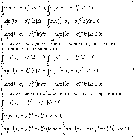 (1)
(1)
|
в
каждом кольцевом сечении оболочки (пластинки) выполняются неравенства
|
the following
inequalities are fulfilled in each annular cross-section of shell (plate)
|
|
в каждом сечении оболочки выполняются
неравенства
|
the following
inequalities are fulfilled in each cross-section of shell
|
Fulfillment of
the last three inequalities in (1) is checked only in cases where at
some points of the shell (plate) the minimum (per cycle) values of the
differences σs = |σφ(e) –
σθ(e)| turn out to be less than the minimum
(per cycle) values of differences σs - |σφ(e)|
and σs - |σθ(e)|.
Symbols  and
and  indicate
that from all (corresponding to different points in time t during the
operating cycle) values, values in brackets, the minimum (maximum) are selected
which then are subject to the wall thickness integration operation;
indicate
that from all (corresponding to different points in time t during the
operating cycle) values, values in brackets, the minimum (maximum) are selected
which then are subject to the wall thickness integration operation;
b) if the inequalities
given in Section 5.5a, are not fulfilled, then the parameters of the
limit cycle can be determined (for cylindrical and spherical shells and round
plates) from the adaptability diagrams (Section 7), constructed for
various types of mechanical loads and temperature fields, as well as various
temperature change programs and loads in time.
In the absence
of a suitable adaptability diagram, the parameters of the limit cycle are
determined by general methods of the theory of adaptability.
5.6. Below is a
description of the general methods for calculating the conditions of
adaptability.
5.6.1. Parameters
of the limit cycle (limit variation ranges of mechanical loads and temperature
fields) are the maximum values of the parameters (in the problem under
consideration), under which the conditions of adaptability given in item 5.6.2
are met, and the minimum values of parameters under which the conditions of
non-adaptability given in item 5.6.5 are met.
5.6.2. The
structure will adapt to external influences if such a distribution of residual
stresses that do not vary in time (satisfying the conditions of equilibrium
under zero external loads) is given, at which the total (including variable
conditional elastic stresses from external influences and constant residual
stresses) reduced (according to the criterion of maximum shear stresses) stresses
do not exceed the limit stresses σs either at one moment of
time or at one of its points.
As applied to
axisymmetric structures, when the directions of the main stresses σφ,
σθ, σz are known and do not change during the
cycle, the conditions of adaptability are formulated as follows:
the structure will adapt
to external influences if such a distribution of time-independent residual
stresses ρφ, ρθ, ρz (satisfying the
equilibrium conditions at zero loads) is specified, which ensures the
fulfillment of inequality for all points of the structure
5.6.3. If there
are mechanical loads which do not change over time (weight of the structure and
attached units, constant hydrostatic pressure, etc.), the latter can be
directly included in the equilibrium conditions mentioned in Section 5.6.2
which shall now be performed not at zero, but at given constant loads.
Accordingly, in terms of adaptability, not residual stresses will appear, but
stresses balanced by constant loads. In this case, the conditional elastic stresses
from the indicated loads need not be calculated.
5.6.4. In case of
violation of the conditions of adaptability, an alternating plastic flow
(usually of a local character) or accumulation of one-sided deformation with
each cycle (progressive form change), covering the whole structure component or
its part, can arise.
The
alternating flow occurs if at least one point of structure cannot be given such
constant stresses at which their sum with conditional elastic stresses from
external influences (referring to the reduced stresses) would not exceed the
stress σs at all times of the cycle. Inter alia, in case when
stresses in the structure vary in proportion to one parameter, an alternating
flow occurs if the magnitude of the conditional elastic stresses exceeds 2σs.
In the absence
of alternating flow, progressive form change will occur if the constant
stresses necessary for the total stresses at each point of the body during the
cycle not to exceed σs do not satisfy the equilibrium
conditions of the structure at given loads that do not vary in time (in the
particular case – at zero loads if there are no permanent external forces).
5.6.5. Along with
the above "static" formulations, the following "kinematic"
formulations can be used to obtain upper assessments of the conditions for the
occurrence of progressive form change. Progressive form change will necessarily
occur if you can specify such (non-zero) distribution of increments for a cycle
of irreversible deformations satisfying the conditions of compatibility of
deformations, during which the work of minimum (per cycle) differences of limit
stresses σs and elastic stresses from external influences (on
the specified increments of irreversible deformations), calculated for the
entire volume of the structural component, is nonpositive.
As applied to
axisymmetric structures, when the directions of the main stresses σφ,
σθ, σz are known and do not change during the
cycle, the condition of existence of progressive form change is formulated as
follows:
progressive form change
takes place if it is possible to set such a distribution of nonzero increments
of plastic deformations per cycle ∆εφ, ∆εθ, ∆εz,
satisfying the compatibility and incompressibility conditions, under which the
inequality is fulfilled
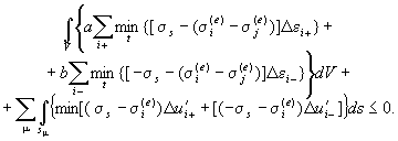
Here a
= 1, b = 0 if two of three components of the deformation increments (∆εφ,
∆εθ, ∆εz) are non-negative; a = 0, b
= 1 if two of three components of the deformation increments (∆εφ,
∆εθ, ∆εz) are negative; index i takes
values of φ, θ, z; index j takes values of φ, θ, z, that
do not match values of i in each sum (therefore, when calculating each
sum, the index can take only one value); ∆u'i is a component
of breakage of increment of displacements on the surface sμ
(in directions of φ, or θ, or z);
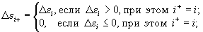
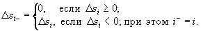
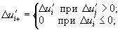
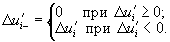
The time-independent
volume (proper weight, inertial forces Xi) or surface
(distributed on sp surfaces) external loads pi
are taken into account by additional additives on the right-hand side of the
inequality, which determines the conditions for existence of a form change:
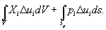
In this case,
the conditional elastic stresses entering the left-hand side of this inequality
are calculated only from external influences varying in time.
5.6.6. Calculation
of the parameters of the limit cycle using items 5.6.2 and 5.6.3
is reduced to finding such a distribution of residual stresses, at which the
parameters of the load or temperature will have maximum values when the
relevant restrictions specified in item 5.6.2 (static calculation
method) are met. Calculation of the parameters of the limit cycle using item 5.6.5
is reduced to minimization of the load (temperature) parameters according to
deformation increments satisfying the restrictions specified in item 5.6.5
(kinematic calculation method).
In the general
case, the specified computational problems are solved by the methods of the
mathematical theory of optimal processes, and when replacing differential
equations of equilibrium (or compatibility of deformations) with a system of
linear algebraic equations – by methods of linear programming using appropriate
standard or special computer sub-programs.
5.6.7. Approximate
lower assessments of the parameters of the limit cycle (i.e., values less than
or equal to the parameters of the limit cycle) are obtained by setting any
distributions of residual stresses that satisfy the equilibrium conditions and
calculating the maximum values of loads and temperatures at which the reduced
stresses (correspond to the sum of residual and conditional elastic stresses)
do not exceed σs.
For example,
it can be assumed that the residual stresses at all points of the structure are
proportional to thermoelastic stresses at one of the cycle moments of time
(this distribution satisfies the equilibrium conditions at zero external loads)
or that some components of the residual stresses (ρφ or ρθ
or ρz) are proportional to the minimum per cycle differences
between σs and corresponding elastic stresses (σφ(e),
σθ(e), σz(e)).
In the latter case, the remaining components of the residual stresses are found
from the equilibrium conditions and then the corresponding lower assessment of
the limit cycle parameters is calculated.
5.6.8. Approximate
upper assessments for the parameters of the limit cycle can be obtained by
using kinematic methods, i.e. methods based on the kinematic theorem (item 5.6.5).
The advantage of these methods is a clear kinematic idea of the nature of the
emerging cyclic plastic deformation, its mechanism. They are used only to
determine the conditions of progressive form change, since the alternating flow
is local and the corresponding limit condition is determined on the grounds of
the above approximate criterion (the change in elastic stresses at the point of
structure exceeds 2σs).
The basis of
the approximate kinematic method lies in the assumption that the distribution
of plastic deformation increments per cycle is possible (satisfying the
conditions of compatibility of deformations). It is usually convenient to find
such a distribution (fracture mechanism) by specifying a certain distribution
of increments of residual displacements at points of the structure, and then
the deformation increments can be calculated using known relations (such as the
Cauchy relation). At the same time, the results of solving similar problems of
limit equilibrium can sometimes be used, since the mechanisms of
"instantaneous" and progressive fracture are generally of the same
type, the difference is in their implementation ("instantly" under
conditions of limit equilibrium and in stages during a cycle with progressive
form change).
It is easiest
to use approximate kinematic methods in axisymmetric problems, since the
distribution of displacement increments here can often be represented as
functions of one coordinate (disk, round plate, tube), sometimes using additional
parameters that are determined during the solution by minimizing the desired
loads. In problems of this type, it is sometimes possible with the help of an
elementary method to obtain exact solutions that satisfy not only kinematic
(the implementation of a certain mechanism of progressive form change), but
also static (no points in which stresses exceed σs during a
cycle) conditions.
For a given
(accepted) fracture mechanism, the parameters of the limit cycle using the
kinematic method are determined using inequalities of the type given in item 5.6.5,
supplemented by members in necessary cases, with due regard to constant
external loads.
The other
version of the kinematic method (the so-called method of additional load)
allows to apply the equilibrium conditions written in the usual form; for this,
the relationship between the plastic deformation increments per cycle and the
effective stresses shall first be used (stresses causing the corresponding
plastic deformation shall reach the yield limit, and the deformation vector
shall be perpendicular to the corresponding face of the hexagon determining the
yield conditions using the maximum shear stress criterion).
5.7. At the
second stage, it is recommended to calculate the kinetics of elastic plastic
deformation if the termination of the progressive form change according to the
data of the first stage is impossible and it is necessary to substantiate the
possibility of the structure operation beyond the limits of adaptability.
At the same
time, it is checked whether progressive form change or its combination with
alternating plastic flow (alternating plastic flow is characterized by the fact
that the plastic deformation increment per cycle is zero) will lead to abnormal
operation of the structure during a given operating life. For this purpose, the
calculated values of deformations are compared with the permissible values
established on the grounds of operational requirements.
When
calculating the deformations, it is necessary to take into account the change
in mechanical characteristics of the material due to alternating plastic flow
(inter alia acceleration of creep due to previous plastic deformation of the
opposite sign, due to neutron exposure, structural transformations, influence
of surface-active media).
In cases where
verification for a progressive form change of a structure by calculation is
difficult, full-size tests or tests on models are recommended.
5.8. In
particular cases for structural components such as rods with a cross-section in
the form of a circle or a regular polygon, thick-walled and thin-walled pipes
of constant thickness with similar cross-sections, free plates with constant
thickness made of the materials listed in Table P4.1 and operating at
thermal cycling in steam water or in sodium at maximum temperatures not exceeding
values of Tf specified in Table P4.1, the accumulated
deformation per cycle does not exceed the values of Δε = 2 · 10-4%
in zones where the edge effect practically does not affect the stress value.
If, for a
given structural component, the deformation accumulated over an operation life
is permissible, further calculations for form changing may not be carried out.
This conclusion is valid under the following conditions:
Table P4.1.
Values of the characteristics of form changing under thermal cycling and
neutron exposure and various media
|
Base metal
and full-strength welds
|
Condition
|
Tf, K (°C)
|
γp,
cm2/(neutron · s)
|
|
Steam
water
|
Sodium, Tmin
= 473 K (200 °C)
|
Sodium, Tmin
= 673 K (400 °C)
|
|
08Kh16N11M3
|
Austenitization
|
773 (500)
|
803 (530)
|
823 (550)
|
4.6 · 10-50
|
|
12Kh18N9
12Kh18N10T
|
"
|
773 (500)
|
803 (530)
|
823 (550)
|
7.6 · 10-50
|
|
08Kh16N11M3
12Kh18N9
12Kh18N10T
|
15% cold-work
hardening + stabilization
|
823 (550)
|
853 (580)
|
853 (580)
|
|
KhN35VT
|
Austenitization +
ageing
|
873 (600)
|
873 (600)
|
873 (600)
|
5.0 · 10-51
|
|
1Kh16N36MBTYUR
|
Austenitization +
stabilization
|
|
10Kh2M 12Kh2M1FB
|
Normalization +
tempering
|
793 (520)
|
823 (550)
|
833 (560)
|
-
|
|
15Kh2MFA
15Kh2NMFA
|
Quenching + tempering
|
793 (520)
|
-
|
-
|
0
|
a) stresses from
mechanical loads are insignificant
(σ)1
≤ 0.1[σ]; (σ)2 ≤ 0.13[σ];
b) temperature of the
medium washing the structure changes all over the volume so quickly that
the gradients in all cross-sections of parts of cylindrical shape
(respectively, for all plate normals) are the same; temperature gradients in
the axial direction (for cylindrical parts) or along the surface (for a plate)
are such that the corresponding thermoelastic stresses are no more than 0.1σs;
c) there are no
conditions that could lead to bending deformation, i.e. the initial shape of
the parts and the temperature fields are strictly symmetrical about the
longitudinal axes (or about the middle plane for the plate); there are no
initial process stresses in the parts, the relaxation of which would lead to
bending; there is no danger of buckling due to thinness of walls.
For the above
structural components at maximum cycle temperatures exceeding the Tf
values given in Table P4.1, but not more than 923 K (650 °C), as well as
for rods and pipes with regular longitudinal stiffeners, undercuts or annular
undercuts with geometrical parameters h1/H ≤ 0.1, ρ ≤ h1/2
with the number of stiffeners or undercuts of no more than 10 and Tmax≤
923 K (650 °C), the upper assessment of the deformation Δε (longitudinal or
transverse without bending) accumulated over one cycle can be found using an
approximate empirical dependence

where T*
= Tf + ∆T0(1 – 10-H/d0)
- ∆Tvχ is a tolerance adjustment temperature 2 · 10-4
%/cycle; ∆T0 = 50 K (50 °C) for rods and thick-walled pipes;
∆T0 = 0 K (0 °C) for plates and thin-walled pipes (shells); H
is a pipe thickness, mm; d0 is a minimum internal diameter of
the pipe (for solid rods d0 = 0), mm; ∆Tv =
-5 K (-5 °C); x is a number of stiffeners or undercuts; h1 is
an undercut depth or stiffener height, mm; ρ is a bending radius, mm; Tmax
is a maximum temperature of thermal cycling, K (°C).
In
non-steady-state modes of thermal cycling, the magnitude of irreversible
deformation is determined by linear summation.
6. EXAMPLE OF CALCULATION
OF CYLINDRICAL CLADDING
6.1. This
example illustrates the order of calculation for progressive form change. In
the example, the structure characteristics and loading parameters are
conventionally selected (inter alia, the simplest one is specified – linear law
of temperature distribution).
6.2. Calculate
the section of the long cylindrical shell (Fig. P4.1), located far from
its edges. The shell is subjected to the action of the inner pressure p(t)
(not varying along its length) and temperature T(t) varying under
linear law along the thickness of the shell at each moment of time t:
T(t) = T0(t)
+ (z/h)T1(t).
Here T0(t)
is a middle surface temperature; T1(t) is a
temperature difference between the outer and middle surfaces of the shell.
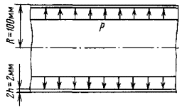
Fig. P4.1.
Section of a long cylindrical shell located far from its edges
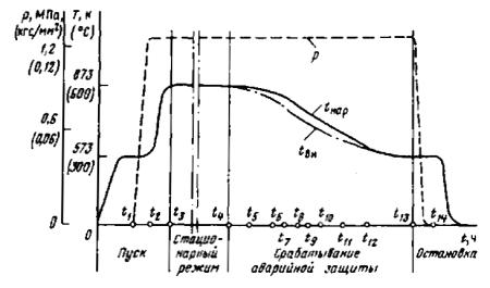
Fig. P4.2.
Changes in pressure and temperature during the operating cycle
|
МПа
|
MPa
|
|
кгс/мм2
|
kgf/mm2
|
|
Пуск
|
Start-up
|
|
Стационарный режим
|
Steady-state mode
|
|
Срабатывание аварийной защиты
|
Emergency protection
actuation
|
|
Остановка
|
Shutdown
|
The purpose of
the calculation is to check the admissibility of given inner pressure and
temperatures of the shell in terms of progressive form change.
6.3. Shell
dimensions are shown in Fig. P4.1. Changes in pressure and temperature
during the operating cycle are shown in Fig. P4.2. In steady-state mode,
in the processes of start-up and shutdown, temperature of the outer and inner
surfaces of the shell To and Ti are assumed
to be the same. Values of T0(t), T1(t)
and p(t) for a number of points in time indicated in Fig. P4.2
are given in Table P4.2.
Mechanical characteristics
of the shell material are given in Table P4.3. At a temperature of 293 K
(20 °C), the modulus of elasticity is E = 2.0 · 105 MPa (2.0
· 104 kgf/mm2), the temperature coefficient of linear
expansion is α = 17 μK-1 (17.0 · 10-6 1/°C) and Poisson
ratio is μ = 0.3. The design operating life of the shell is 100000 hours.
6.4. Determine
the ultimate stresses σs:
a) for steady-state
operation mode in accordance with Section 3.2.
σs
= min{RTp0.2/n0.2; RTmt/nmt}
= min{120/1.5; 125/1.5} = 80.0 MPa (8.0 kgf/mm2);
Table P4.2. Loading
parameters
|
t
|
t1
|
t2
|
t3
|
t4
|
t5
|
t6
|
t7
|
|
T0,
|
K
(°C)
|
573
(300)
|
573
(300)
|
873
(600)
|
873
(600)
|
856
(583)
|
867.5
(594.5)
|
794
(521)
|
|
T1,
|
K
(°C)
|
273
(0)
|
273
(0)
|
273
(0)
|
273
(0)
|
277.5
(4.50)
|
284.25
(11.25)
|
289.56
(16.56)
|
|
p,
|
MPa
(kgf/mm2)
|
0
0
|
1.2
(0.12)
|
1.2
(0.12)
|
1.2
(0.12)
|
1.2
(0.12)
|
1.2
(0.12)
|
1.2
(0.12)
|
Table P4.2 (continued)
|
t
|
t8
|
t9
|
t10
|
t11
|
t12
|
t13
|
t14
|
|
T0,
|
K
(°C)
|
765.5
(492.5)
|
734
(461)
|
709
(436)
|
667
(394)
|
639
(366)
|
573
(300)
|
573
(300)
|
|
T1,
|
K
(°C)
|
292.55
(19.55)
|
293
(20.00)
|
289.56
(16.56)
|
285
(12.00)
|
281.75
(8.75)
|
273
(0)
|
273
(0)
|
|
p,
|
MPa
(kgf/mm2)
|
1.2
(0.12)
|
1.2
(0.12)
|
1.2
(0.12)
|
1.2
(0.12)
|
1.2
(0.12)
|
1.2
(0.12)
|
0
0
|
Table P4.3. Mechanical
characteristics of the shell material
|
T,
|
K
(°C)
|
293
(20)
|
573
(300)
|
623
(350)
|
673
(400)
|
723
(450)
|
773
(500)
|
823
(550)
|
873
(600)
|
|
RTp0.2
|
MPa
(kgf/mm2)
|
210
(21)
|
150
(15)
|
150
(15)
|
140
(14)
|
140
(14)
|
130
(13)
|
120
(12)
|
120
(12)
|
|
R1/100000,
|
MPa
(kgf/mm2)
|
-
|
-
|
-
|
-
|
181
(18.1)
|
169
(16.9)
|
137
(13.7)
|
100
(10.0)
|
b) limit stresses for
start-up, emergency protection actuation and shutdown modes found according to
Section 3.1
σs
= (RTp0.2/1.5)
are given depending on
the temperature in Table P4.4.
6.5. Determine
the conditional elastic stresses in the operating cycle. Ring stresses from
inner pressure σθp at p = 1.2 MPa (0.12 kgf/mm2)
(see Fig. P4.2) are equal to 60 MPa (6 kgf/mm2), axial stress
from mechanical load is zero.
Table P4.4.
Limit stresses
|
T, K (°C)
|
293 (20)
|
573 (300)
|
623 (350)
|
673 (400)
|
723 (450)
|
773 (500)
|
823 (550)
|
873 (600)
|
|
σs,
MPa
(kgf/mm2)
|
140.0
(14.00)
|
100.0
(10.00)
|
100.0
(10.00)
|
93.3
(9.33)
|
93.3
(9.33)
|
86.7
(8.67),
|
80.0
(8.00)
|
80.0
(8.00)
|
Table P.4.5. Thermoelastic
stresses
|
t
|
t4
|
t5
|
t6
|
t7
|
t8
|
t9
|
t10
|
t11
|
t12
|
t13
|
|
σθT
= σφT, MPa
(kgf/mm2)
|
0
(0)
|
21.8
(2.18)
|
54.6
(5.46)
|
80.4
(8.04)
|
95.0
(9.50)
|
97.1
(9.71)
|
80.4
(8.04)
|
58.3
(5.83)
|
42.5
(4.25)
|
0
(0)
|
Thermoelastic
stresses when a linear temperature distribution across the wall thickness are
found using the formula
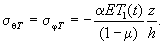
Here σθT,
σφT are annular and axial thermoelastic stresses; z
coordinate is measured from the middle surface of the shell along the normal to
it; z = h on the outer surface of the shell and z = -h
on the inner surface.
In a
steady-state mode, at start-up and shutdown, thermoelastic stresses are zero
[because T1(t) = 0]. Values of stresses σθT
= σφT for a number of points in time of the mode of emergency
protection actuation are given in Table P4.5 for points lying on the
inside (z = -h) surface of the shell.
6.6. Compare the
above conditional elastic stresses with limit stresses. Reduced conditional
elastic stresses are calculated according to the criterion of the greatest
shear stresses:
(σ)(e)
= max(|σφ(e)|, |σθ(e)|,
|σφ(e) - σθ(e)|),
where σθ(e)
= σθT + σθT; σφ(e)
= σφp + σφT = σφT.
In the moment
of time t9 on the inner surface of the shell (σ)(e)
= 60.0 + 97.1 = 157.1 MPa (15.71 kgf/mm2). The temperature of the
points of the inner surface of the shell at this moment determined according to
the data in Table P4.1 is 714 K (441 °C); the corresponding limit stress
σs found from the data in Table P4.3 using linear
interpolation is 93.3 MPa (9.33 kgf/mm2). Thus, the reduced stress
(σ)(e) exceeds the limit one. It is not necessary to compare
the reduced stresses with the limit ones at other points of the shell and at
other moment of times, since the result obtained above requires a transition to
the next stage of calculation: verification whether plastic deformation can
stop due to the redistribution of stresses across the shell thickness.
6.7. Determine
the extremal values of the difference of limit and conditional elastic
stresses. To check whether the inequalities written in item 5.5a are
satisfied, we calculate the values
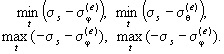
Table P4.6. Difference
of limit and conditional elastic stresses
|
Mode
|
Start-up
|
Steady-state
|
Shutdown
|
|
t
|
t1
|
t2
|
t3
|
t4
|
t13
|
t14
|
|
T, K (°C)
|
573 (300)
|
573 (300)
|
873 (600)
|
873 (600)
|
573 (300)
|
573 (300)
|
|
σs,
MPa, (kgf/mm2)
|
100 (10)
|
100 (10)
|
80 (8)
|
80 (8)
|
100 (10)
|
100 (10)
|
|
σs -
σφ(e), MPa (kgf/mm2)
|
100 (10)
|
100 (10)
|
80 (8)
|
80 (8)
|
100 (10)
|
100 (10)
|
|
-σs
- σφ(e), MPa (kgf/mm2)
|
-100 (-10)
|
-100 (-10)
|
-80 (-8)
|
-80 (-8)
|
-100 (-10)
|
-100 (-10)
|
|
σs –
σθ(e), MPa (kgf/mm2)
|
100 (10)
|
40 (4)
|
20 (2)
|
20 (2)
|
40 (4)
|
100 (10)
|
|
-σs –
σθ(e), MPa (kgf/mm2)
|
-100 (-10)
|
-160 (-16)
|
-140 (-14)
|
-140 (-14)
|
-16 (-160)
|
-100 (-10)
|
The values in
brackets for the steady-state mode and a number of time moments for the
start-up and shutdown modes [those in which T1(t) = 0]
are given in Table P4.6. According to the shell thickness, these values
do not change for the specified modes. Extreme values for these modes of the
considered quantities are enclosed in frames [it is easy to verify that at Т1(t)
= 0 at time moments not listed in Table P4.6 extreme values are not
reached].
Next, we find
the difference between the limit and conditional elastic stresses for a number
of moments of the mode of the emergency protection actuation (T1(t)
≠ 0). To determine the extremal values of these differences, it is sufficient
to consider the moments of time t9, t8, t7,
t4 and the conditional elastic and limit stresses at time t4
coincide with the corresponding values at time t3 (see Table P4.6).
At time moments t10, t11 and t12,
the conditional elastic stresses decrease and the limit stresses increase in
comparison with t9 (see Tables P4.1, P4.3 and P4.4),
therefore, the indicated moments in time are not considered. The calculation
results are given in Table P4.6.
To preserve
the generality of the procedure in Table P4.6 the temperature dependence
of the limit stresses σs is considered. Due to the small
temperature differences across the thickness in this example, this dependence
has little effect on the calculation results, however, in other problems (inter
alia, when parabolic laws of temperature distribution) it sometimes turns out
to be significant.
The
calculation of differences of limit and elastic stresses for a number of
moments in time is shown in Fig. P4.3 and P4.4; bold lines
indicate the corresponding minimum (maximum) values per cycle.
The values of
differences of limit and conditional elastic stresses over the entire operating
cycle are given in Tables P4.6 and P4.7, and the extreme values
of these differences are given in Table P4.8.
6.8. Fulfillment
of the conditions for the absence of progressive form change, given in Section 5.5a,
is verified by numerical integration using the data in Table P4.8:
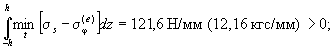
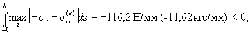


Fig. P4.3.
Values of stress differences at different moments of time for σs
- σφ(e) (a) and –σs - σφ(e)
(b)
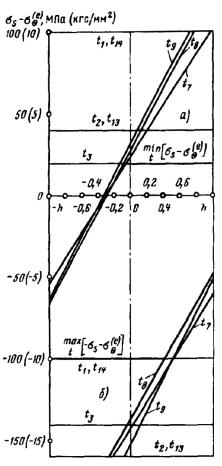
Fig. P4.4.
Values of stress differences at different moments of time for σs
– σθ(e) (a) and –σs
– σθ(e) (b)

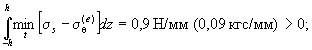
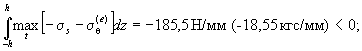


As a result,
we come to the conclusion that there will be no progressive form change of the
shell under the specified operating conditions.
7. ADAPTABILITY DIAGRAMS
FOR SOME STANDARD DESIGN MODELS
7.1. Formulas
and diagrams of adaptability for cylindrical and spherical shells, thick-walled
spherical vessels and round plates under repeated mechanical and thermal
effects are given below. The diagrams are constructed for various types of
mechanical loads (distributed, concentrated) and temperature fields
(temperature varies in thickness along the generatrix), various programs for
changing temperature and loads over time, as well as for different conditions
for fixing the shell or plate. Provided that it is assumed that σs
= const and μ = 0.3.
General symbols:
T is a temperature, K (°C);
p is a
pressure, Pa (kgf/mm2);
P is a concentrated force, N (kgf);
n, m, f,
q are load parameters;
tp are
temperature parameters;
R is radius of the middle surface of the shell
(radius of the plate), mm;
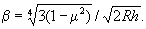
The formulas
and diagrams given here can be used in cases where the loads, temperatures and
geometrical characteristics of the component of structure correspond to the
conditions for which the corresponding graphs and formulas are given.
To use
formulas and diagrams, it is necessary to calculate the parameters of
mechanical and thermal effects m, p, q, n, tp
for given structure and operation conditions and compare their values with the
limit values indicated on the diagram or calculated using the formula given
here. The structure will adapt to the specified external influences if the
parameters of the loads and the temperature that meet the specified operation
conditions do not exceed the limit values.
Table P4.7. Differences
of limit and conditional elastic stresses depending on z/h
|
|
z/h
|
-1.0
|
-0.8
|
-0.6
|
-0.4
|
-0.2
|
0
|
0.2
|
0.4
|
0.6
|
0.8
|
1.0
|
|
t9
|
T, K (°C)
|
714
(441)
|
718
(445)
|
722
(449)
|
726
(453)
|
730
(457)
|
734
(461)
|
738
(465)
|
742
(469)
|
746
(473)
|
750
(477)
|
754
(481)
|
|
σs,
MPa
(kgf/mm2)
|
93.3
(9.33)
|
93.3
(9.33)
|
93.3
(9.33)
|
92.6
(9.26)
|
92.4
(9.24)
|
91.8
(9.18)
|
91.3
(9.13)
|
90.8
(9.08)
|
90.3
(9.03)
|
89.7
(8.97)
|
89.2
(8.92)
|
|
σφ(e),
MPa
(kgf/mm2)
|
97.1
(9.71)
|
77.7
(7.77)
|
58.3
(5.83)
|
38.8
(3.88)
|
19.4
(1.94)
|
0
(0)
|
-19.4
(-1.94)
|
-38.8
(-3.88)
|
-58.3
(-5.83)
|
-77.7
(-7.77)
|
-97.1
(-9.71)
|
|
σs -
σφ(e), MPa
(kgf/mm2)
|
-3.8
(-0.38)
|
15.6
(1.56)
|
35.0
(3.50)
|
53.8
(5.38)
|
73.0
(7.30)
|
91.8
(9.18)
|
110.7
(11.07)
|
129.6
(12.96)
|
148.6
(14.86)
|
167.4
(16.74)
|
186.3
(18.63)
|
|
-σs
- σφ(e), MPa
(kgf/mm2)
|
-190.4
(-19.04)
|
-171.0
(-17.10)
|
-151.6
(-15.16)
|
-131.4
(-13.14)
|
-111.8
(-11.18)
|
-91.8
(-9.18)
|
-71.9
(-7.19)
|
-52.0
(-5.20)
|
-32.0
(-3.20)
|
-12.0
(-1.20)
|
7.9
(0.79)
|
|
σθ(e),
MPa
(kgf/mm2)
|
157.1
(15.71)
|
137.7
(13.77)
|
118.3
(11.83)
|
98.8
(9.88)
|
79.4
(7.94)
|
60.0
(6.00)
|
40.6
(4.06)
|
21.8
(2.18)
|
1.7
(0.17)
|
-17.7
(-1.77)
|
-37.1
(-3.71)
|
|
σs –
σθ(e), MPa
(kgf/mm2)
|
-63.8
(-6.38)
|
-44.4
(-4.44)
|
-25.0
(-2.50)
|
-6.2
(-0.62)
|
13.0
(1.30)
|
31.8
(3.18)
|
50.7
(5.07)
|
69.6
(6.96)
|
88.6
(8.86)
|
107.6
(10.76)
|
126.3
(12.63)
|
|
-σs
– σθ(e), MPa
(kgf/mm2)
|
-250.4
(-25.04)
|
-231.0
(-23.10)
|
-211.6
(-21.16)
|
-191.4
(-19.14)
|
-171.8
(-17.18)
|
-151.8
(-15.18)
|
-131.9
(-13.19)
|
-112.0
(-11.20)
|
-92.0
(-9.20)
|
-72.0
(-7.20)
|
-52.1
(-5.21)
|
|
t10
|
T, K (°C)
|
746
(473)
|
750
(477)
|
754
(481)
|
758
(485)
|
762
(489)
|
765.5
(492.5)
|
769
(496)
|
773
(500)
|
777
(504)
|
781
(508)
|
785
(512)
|
|
σs,
MPa
(kgf/mm2)
|
90.3
(9.03)
|
89.7
(8.97)
|
89.2
(8.92)
|
88.7
(8.87)
|
88.2
(8.82)
|
87.7
(8.77)
|
87.2
(8.72)
|
86.7
(8.67)
|
86.2
(8.62)
|
85.6
(8.56)
|
85.1
(8.51)
|
|
σφ(e),
MPa
(kgf/mm2)
|
95.0
(9.50)
|
76.0
(7.60)
|
57.0
(5.70)
|
38.0
(3.80)
|
19.0
(1.90)
|
0
(0)
|
-19.0
(-1.90)
|
-38.0
(-3.80)
|
-57.0
(-5.70)
|
-76.0
(-7.60)
|
-95.0
(-9.50)
|
|
σs -
σφ(e), MPa
(kgf/mm2)
|
-4.7
(-0.47)
|
13.7
(1.37)
|
32.2
(3.22)
|
50.7
(5.07)
|
69.2
(6.92)
|
87.7
(8.77)
|
106.2
(10.62)
|
124.7
(12.47)
|
143.2
(14.32)
|
161.6
(16.16)
|
180.1
(18.01)
|
|
-σs
- σφ(e), MPa
(kgf/mm2)
|
-185.3
(-18.53)
|
-165.7
(-16.57)
|
-146.2
(-14.62)
|
-126.7
(-12.67)
|
-107.2
(-10.72)
|
-87.7
(-8.77)
|
-68.2
(-6.82)
|
-48.7
(-4.87)
|
-29.2
(-2.92)
|
-9.6
(-0.96)
|
9.9
(0.99)
|
|
σθ(e),
MPa
(kgf/mm2)
|
155.0
(15.55)
|
136.0
(13.60)
|
117.0
(11.70)
|
98.0
(9.80)
|
79.0
(7.90)
|
60.0
(6.00)
|
41.0
(4.10)
|
22.0
(2.20)-
|
3.0
(0.30)
|
16.0
(1.60)
|
-35.0
(-3.50)
|
|
σs –
σθ(e), MPa
(kgf/mm2)
|
-64.7
(-6.47)
|
-46.3
(-4.63)
|
-27.8
(-2.78)
|
-9.3
(-0.93)
|
9.2
(0.92)
|
27.7
(2.77)
|
46.2
(4.62)
|
64.7
(6.47)
|
83.2
(8.32)
|
101.6
(10.16)
|
120.1
(12.01)
|
|
-σs
– σθ(e), MPa
(kgf/mm2)
|
-245.3
(-24.53)
|
-225.3
(-22.53)
|
-266.2
(-26.62)
|
-186.7
(-18.67)
|
-167.2
(-16.72)
|
-147.7
(-14.77)
|
-128.2
(-12.82)
|
-108.7
(10.87)
|
-89.2
(-8.92)
|
-69.6
(-6.96)
|
-50.1
(-5.01)
|
|
t11
|
T, K (°C)
|
777
(504)
|
781
(508)
|
784
(511)
|
787
(514)
|
791
(518)
|
794
(521)
|
797
(524)
|
801
(528)
|
804
(531)
|
807
(534)
|
811
(538)
|
|
σs,
MPa
(kgf/mm2)
|
86.2
(8.62)
|
85.6
(8.56)
|
85.2
(8.52)
|
84.8
(8.48)
|
84.3
(8.43)
|
83.9
(8.39)
|
83.5
(8.35)
|
82.9
(8.29)
|
82.5
(8.25)
|
82.1
(8.21)
|
81.6
(8.16)
|
|
σφ(e),
MPa
(kgf/mm2)
|
80.4
(8.04)
|
64.3
(6.43)
|
48.2
(4.82)
|
32.2
(3.22)
|
16.1
(1.61)
|
0
(0)
|
-16.1
(-1.61)
|
-36.6
(-3.66)
|
-48.2
(-4.82)
|
-64.3
(-6.43)
|
-80.4
(-8.04)
|
|
σs -
σφ(e), MPa
(kgf/mm2)
|
5.8
(0.58)
|
21.3
(2.13)
|
37.0
(3.70)
|
52.6
(5.26)
|
68.2
(6.82)
|
89.3
(8.93)
|
99.6
(9.96)
|
115.1
(11.51)
|
130.7
(13.07)
|
146.4
(14.64)
|
162.0
(16.20)
|
|
-σs
- σφ(e), MPa
(kgf/mm2)
|
-166.6
(-16.66)
|
-149.9
(-14.99)
|
-133.4
(-13.34)
|
-117.0
(-11.70)
|
-100.4
(-10.04)
|
-83.9
(-8.39)
|
-67.4
(-6.74)
|
-50.7
(-5.07)
|
-34.3
(-3.43)
|
-17.8
(-1.78)
|
-1.2
(-0.12)
|
|
σθ(e),
MPa
(kgf/mm2)
|
140.4
(14.04)
|
124.3
(12.43)
|
108.2
(10.82)
|
92.2
(9.22)
|
76.1
(7.61)
|
60.0
(6.00)
|
43.9
(4.39)
|
27.8
(2.78)
|
11.8
(1.18)
|
-4.3
(-0.43)
|
-20.4
(-2.04)
|
|
σs –
σθ(e), MPa
(kgf/mm2)
|
-54.2
(-5.42)
|
-38.7
(-3.87)
|
-23.0
(-2.30)
|
-7.4
(-0.74)
|
8.2
(0.82)
|
23.9
(2.39)
|
39.6
(3.96)
|
55.1
(5.51)
|
70.7
(7.07)
|
86.4
(8.64)
|
102.0
(10.20)
|
|
-σs
– σθ(e), MPa
(kgf/mm2)
|
-226.6
(-22.66)
|
-209.9
(-20.99)
|
-193.4
(-19.34)
|
-167.0
(-16.70)
|
-160.4
(-16.04)
|
-143.9
(-14.39)
|
-127.4
(-12.74)
|
-110.7
(-11.07)
|
-94.3
(-9.43)
|
-77.8
(-7.78)
|
-61.2
(-6.12)
|
Table P4.8. Extreme
values of stress differences
|
z/h
|
-1.0
|
-0.8
|
-0.6
|
-0.4
|
-0.2
|
0
|
0.2
|
0.4
|
0.6
|
0.8
|
1.0
|
|
 , MPa (kgf/mm2) , MPa (kgf/mm2)
|
-4.7
(-0.47)
|
13.7
(1.37)
|
32.2
(3.22)
|
50.7
(5.07)
|
68.2
(6.82)
|
80.0
(8.00)
|
80.0
(8.00)
|
80.0
(8.00)
|
80.0
(8.00)
|
80.0
(8.00)
|
80.0
(8.00)
|
|
 , MPa (kgf/mm2) , MPa (kgf/mm2)
|
-80.0
(-8.00)
|
-80.0
(-8.00)
|
-80.0
(-8.00)
|
-80.0
(-8.00)
|
-80.0
(-8.00)
|
-80.0
(-8.00)
|
-67.4
(-6.74)
|
-48.7
(-4.87)
|
-29.2
(-2.92)
|
-9.6
(-0.96)
|
9.9
(0.99)
|
|
 , MPa (kgf/mm2) , MPa (kgf/mm2)
|
-64.7
(-6.47)
|
-46.3
(-4.63)
|
-27.8
(-2.78)
|
-9.3
(-0.93)
|
8.2
(0.82)
|
20.0
(2.00)
|
20.0
(2.00)
|
20.0
(2.00)
|
20.0
(2.00)
|
20.0
(2.00)
|
20.0
(2.00)
|
|
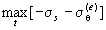 , MPa
(kgf/mm2) , MPa
(kgf/mm2)
|
-100.0
(-10.00)
|
-100.0
(-10.00)
|
-100.0
(-10.00)
|
-100.0
(-10.00)
|
-100.0
(-10.00)
|
-100.0
(-10.00)
|
-100.0
(-10.00)
|
-100.0
(-10.00)
|
-89.2
(-8.92)
|
-69.6
(-6.96)
|
-50.1
(-5.01)
|
When using the
formulas and diagrams below, the calculation of the form change conditions
according to Section 5 are not carried out.
7.2. Cylindrical
vessels and pipelines are loaded with constantly acting pressure and cyclically
varying temperature (pressure and temperature do not change along the axis),
material creep is absent. The limit values of the range of temperature stresses
are determined from the following relations:
a) with a linear
temperature variation along the thickness
 for
for 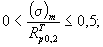
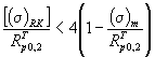 for
for 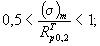
b) with a parabolic
constant increase or decrease in temperature along the wall thickness
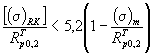 when
when 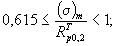
if  then
then
 when
when 
 when
when 
 when
when 
For
intermediate values of (σ)m/RTp0.2,
linear interpolation is allowed.
7.3. Cylindrical
pipe (Fig. P4.5) is exposed to temperature front (Fig. P4.6 - P4.8).
The temperature front moves in any direction along the pipe axis. The
temperature does not change along the pipe thickness.
Repeated flows
of the temperature front shown in Fig. P4.6 lead to a decrease in pipe
diameter and an increase in its length with 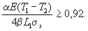

|
Fig. P4.5. The section of
the cylindrical pipe away from the edges
|
Fig. P4.6.
Temperature front leading to a reduction in pipe diameter
|
Repeated flows
of the temperature front shown in Fig. P4.7 lead to a increase in pipe
diameter and an decrease in its length with 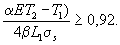
If 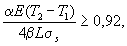 , repeated
flows of the temperature front shown in Fig. P4.8 make the pipe behavior
unstable. A change in the nature of the T(x) dependence or a
change in the limit stress σs leads either to an increase or
to a decrease in the pipe diameter after each flow of the temperature front.
, repeated
flows of the temperature front shown in Fig. P4.8 make the pipe behavior
unstable. A change in the nature of the T(x) dependence or a
change in the limit stress σs leads either to an increase or
to a decrease in the pipe diameter after each flow of the temperature front.
7.4. A finite
length cylindrical shell (Fig. P4.9) is loaded with inner pressure and
temperature difference across the wall thickness
0 ≤ p(t) ≤ p*;
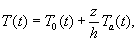
where 
 -T ≤ Ta(t)
≤ T1; -h ≤ z ≤ h.
-T ≤ Ta(t)
≤ T1; -h ≤ z ≤ h.
Loading
parameters tp = EαT/[(1 - μ)σs]; f = p*R/[2hσs]; - tp
≤ tp(t) ≤ tp; 0 ≤ f(t)
≤ f.
Diagrams of
adaptability of a finite length cylindrical shell with free edges are shown in
Fig. P4.10, with simply supported edges – in Fig. P4.11, P4.12,
with clamped edges – in
Fig. P4.13 - P4.15.
7.5. Cylindrical
shell (Fig. P4.16) is loaded with inner pressure and temperature difference
across the wall thickness; on the edge, edge bending moment M(t)
and shear force Q(t) are applied:
0 ≤ p(t) ≤ p*; 0
≤ M(t) ≤ M;
0 ≤ Q(t) ≤ Q;
where -T
≤ Ta(t) ≤ T; -h ≤ z ≤ h.
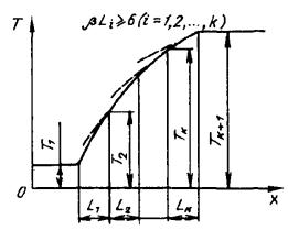
Fig. P4.7.
Temperature front leading to a decrease in pipe diameter
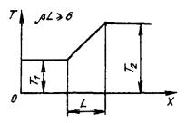
Fig. P4.8.
Temperature front causing unstable pipe behavior
Loading
parameters:


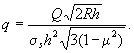
Diagrams of adaptability
for the edge of a cylindrical shell for different values of the parameters f
and tp are shown in Fig. P4.17 - P4.20.
7.6. Long
cylindrical shell (Fig. P4.21) is loaded with a force P
distributed over a circular cross-section and a temperature difference across
the wall thickness:
P = const; 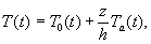
where 
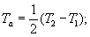 -T
≤ Ta(t) ≤ T; -h ≤ z ≤ h.
-T
≤ Ta(t) ≤ T; -h ≤ z ≤ h.
Loading
parameters:


Diagrams of
adaptability are shown in Fig. P4.22.
7.7. Closed
spherical shell (Fig. P4.23) is loaded with inner pressure and
temperature difference across the wall thickness:
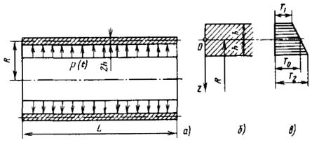
Fig. P4.9. A
finite length cylindrical shell:
a is a shell
loaded with inner pressure; b is a shell cross-section; c is a
temperature difference

Fig. P4.10.
Diagrams of adaptability for a finite length cylindrical shell with free edges
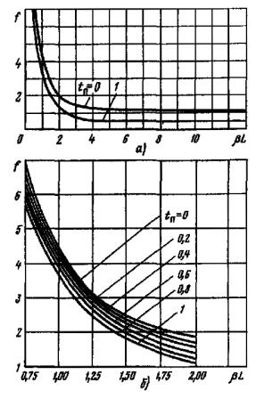
Fig. P4.11.
Diagrams of adaptability for a finite length cylindrical shell with simply
supported edges:
a – general
view of diagrams; b – for βL = 0.75 ÷ 2.00
0 ≤ p(t) ≤ p*;
where -T
≤ Ta(t) ≤ T; -h ≤ z ≤ h.
Loading
parameters:

Fig. P4.12.
Diagrams of adaptability for a finite length cylindrical shell with simply
supported edges
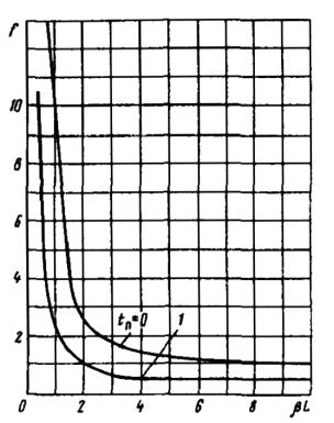
Fig. P4.13.
General view of diagrams of adaptability for a finite length cylindrical shell
with clamped edges
f = p*R/(4σsh);
tp = αET/(1 - μ)σs.
Diagrams of
adaptability for a closed spherical shell are shown in Fig. P4.24.
7.8. Supported
spherical shell (Fig. P4.25) is loaded with inner pressure and temperature
difference across the wall thickness:
p* = const;
where -T
≤ Ta ≤ T; -h ≤ z ≤ h.
Loading
parameters:
f = p*R/(4σsh);
tp = EαT/[2(1 - μ)σs].
Fig. P4.26
shows diagrams of adaptability for the supported spherical shell (2h/R
= 1/20).
7.9. Clamped
spherical shell (Fig. P4.27) is loaded with inner pressure and
temperature difference across the wall thickness:
p* = const; 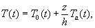
where -T
≤ Ta ≤ T; -h ≤ z ≤ h.
For parameters
of loading and temperature difference see Section 7.8.
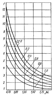
Fig. P4.14.
Diagrams of adaptability for a finite length cylindrical shell with clamped
edges for βL = 0.75 ÷ 2.00
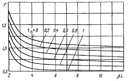
Fig. P4.15.
Diagrams of adaptability for a finite length cylindrical shell with clamped
edges βL = 2 ÷ 12
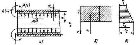
Fig. P4.16.
Edge of the cylindrical shell:
a are loads at
the shell edge; b is a shell cross-section; c is a temperature
difference
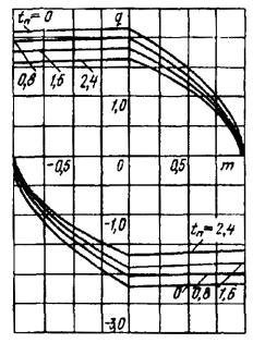
Fig. P4.17.
Diagrams of adaptability for the edge of a cylindrical shell at f = 0
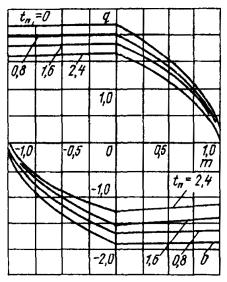
Fig. P4.18.
Diagrams of adaptability for the edge of a cylindrical shell f = 0.25
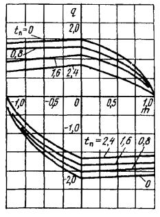
Fig. P4.19.
Diagrams of adaptability for the edge of a cylindrical shell f = 0.5
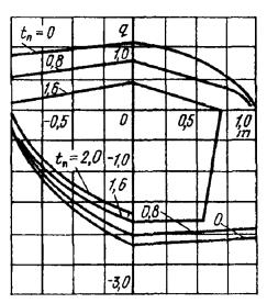
Fig. P4.20.
Diagrams of adaptability for the edge of a cylindrical shell f = 0.75
Fig. P4.28
shows diagrams of adaptability for a clamped spherical shell.
7.10.
Thick-walled closed spherical vessel is loaded with inner pressure p*
= const and temperature difference across the wall thickness:
T(t, ρ) = Tb(t)
+ ∆T(t)k(1 - ρ)/ρ(1 - k),
where ∆T(t) = Tb(t)
- Ta(t); ∆T- ≤ ∆T(t) ≤
∆T+; ∆T = ∆T+ - ∆T-;
k = a/b;
ρ = r/b;
Tb(t) is an outer
surface temperature, Ta(t) is an inner surface
temperature; r is a current radius; b is an outer radius; a
is an inner radius.
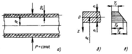
Fig. P4.21.
Long cylindrical shell:
a is a shell
loaded by a force P distributed over a circular section; b is a
shell cross-section; c is a temperature difference
Loading
parameters:
tp = αE∆T/[2(1
– μ)σs]; f = p*/σs.
Fig. P4.29
shows the diagrams of adaptability for a spherical thick-walled vessel for a
number of values k.
7.11. Round
freely supported plate (Fig. P4.30) loaded with uniformly distributed
pressure and temperature field:
0 ≤ p(t) ≤ p*; 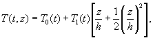
where 0 ≤ T1(t)
≤ T1; min T0 ≤ T0(t)
≤ max T0.
Loading
parameters:
f = p*R2/(6σsh2);
tp = αET1/[6(1 – μ)σs].
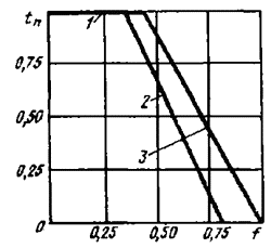
Fig. P4.22.
Diagrams of adaptability for a long cylindrical shell, loaded by a force
distributed across a circular cross-section and temperature difference
distributed across the wall thickness:
1 is an alternating flow;
2 is a progressive form change under the condition of fluidity: max(|mx0|
+ 2tp/3; |nφ0| + |mx0|/2
+ tp/2) = 1; 3 is a progressive form change under the
condition of fluidity: max(|mx0| + 2tp/3;
|nφ0| + tp/2) = 1. (Solution of
the problem of progressive form change under the condition of fluidity
according to the theory of maximum shear stresses lies between lines 2 and 3)
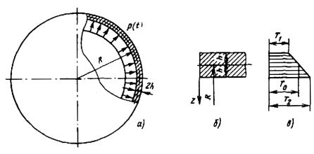
Fig. P4.23.
Closed spherical shell:
a is a shell
loaded with inner pressure; b is a shell cross-section; c is a
temperature difference
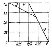
Fig. P4.24.
Diagrams of adaptability for a closed spherical shell:
1 is an alternating flow
at p(t) = const; 2 is an alternating flow with arbitrary
loading program; 3 is a progressive form change p(t) =
const
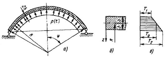
Fig. P4.25.
Supported spherical shell:
a is a shell
loaded with inner pressure; b is a shell cross-section; c is a
temperature field
Fig. P4.31
gives diagrams of adaptability for a round simply supported plate loaded with
uniformly distributed pressure and temperature field.
7.12. Round
freely supported plate (Fig. P4.32) is loaded with alternately
distributed pressure and bending moment:
0≤ p(t) ≤ p*;
0 ≤ M(t) ≤M.
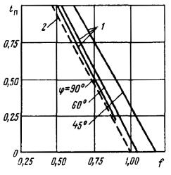
Fig. P4.26.
Diagrams of adaptability for the supported spherical shell (2h/R
= 1/20):
1 is an upper assessment
of the progressive form change condition; 2 is a lower assessment of the
progressive form change condition
Fig. P4.27.
Clamped spherical shell
Fig. P4.28.
Diagrams of adaptability for clamped spherical shell at 2h/R =
1/20 (a) and 2h/R = 1/40 (b):
1 is an upper assessment
of the progressive form change condition; 2 is a lower assessment
Loading
parameters:
f = p*R2/(6σsh2);
m = M/(σsh2).
Fig. P4.33
gives diagram of adaptability for a round simply supported plate loaded with
alternately distributed pressure and bending moment.
7.13. The round
plate, clamped along the edge, is loaded with uniformly distributed pressure
and temperature field (Fig. P4.34). The pressure varies within the
following limits: 0 ≤ p(t) ≤ p*; pressure
loading parameter f = p*R2/(11.26σsh2).
Fig. P4.29.
Diagrams of adaptability for a spherical thick-walled vessel with p =
const:
1 is an alternating flow;
2 is a progressive form change
Fig. P4.30.
Round simply supported plate loaded with uniformly distributed pressure
(supports do not prevent radial displacement)
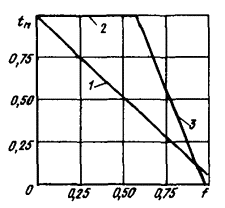
Fig. P4.31.
Diagrams of adaptability for a round simply supported plate loaded with
uniformly distributed pressure and temperature field:
1 is an alternating flow
with an arbitrary loading program: (15/16)f + tp = 1; 2
is an alternating flow at p(t) = const, tp = 1;
3 is a progressive form change at p(t) = const, f +
(5/12)tp = 1
Fig. P4.35
and P4.36 shows diagrams of adaptability for a round plate clamped along
the edge for the following temperature fields:
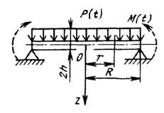
Fig. P4.32.
Round simply supported plate loaded with alternately distributed pressure and
bending moment
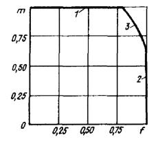
Fig. P4.33.
Diagram of adaptability for a round simply supported plate loaded with
alternately distributed pressure and bending moment:
1 is an
"instant" plastic destruction m = 1; 2 is an
"instant" plastic destruction f = 1; 3 is a progressive
form change m(1 - x) + (1/4)(5 – x2)x =
1; x2 = (1/3)(5 - 4mf)
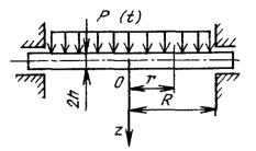
Fig. P4.34.
Round plate clamped along the edge
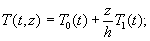 0 ≤ T1(t)
≤ T1;
0 ≤ T1(t)
≤ T1;
min T0 ≤ T0(t)
≤ max T0; temperature parameter t = αET1/[2×(1 - μ)σs] (Fig. P4.35);

0 ≤ T1(t)
≤ T1; temperature parameter tp = 2αET1/[3(1 - μ)σs] (Fig. P4.36).
7.14. Simply
supported round plate (Fig. P4.37) is loaded with force P =
const, distributed over the ring, and the temperature field.
Loading
parameters:
f = Pa/(σsh2);
tp = αET1/σs.
Fig. P4.38,
P4.39 shows diagrams of adaptability for a simply supported round plate
with a force distributed over the ring for the following temperature fields:
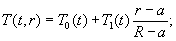 (Fig. P4.38)
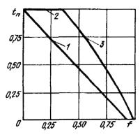
Fig. P4.35.
Diagrams of adaptability for a round plate, clamped along the edge, with 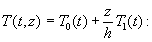
1 is an alternating flow
with an arbitrary loading program: 1.055f + tp = 1; 2
is an alternating flow at p* = const, tp =
1; 3 is a progressive form change at p(t) = const, -0 ≤ tp
≤ 0.75; f = 0.533x2; 3x2 – 2ln
x – 5 – (8/3)tp; -0.75 ≤ tp ≤ 1.0; f
= 1.066(1 – (2/3)tp)

Fig. P4.36.
Diagrams of adaptability for a round plate, clamped along the edge, with 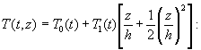
1 is an alternating flow
with an arbitrary loading program: 1.055f + tp = 1; 2
is an alternating flow at p(t) = const, tp = 1;
3 is a progressive form change at p(t) = const, f =
0.535x2;
3x2 – 2ln x - 5 = -2tp
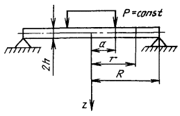
Fig. P4.37.
Simply supported round plate with force distributed over the ring
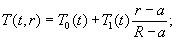 (Fig. P4.39);
Hre at a ≤
r ≤ R 0 ≤ T1(t) ≤ T1;
at 0 ≤ r ≤ a T1(t)
=0;
min T0≤
T0(t) ≤ max T0; k = a/R.
7.15. Simply
supported round plate with a stepwise change in thickness (Fig. P4.40)
is loaded with concentrated force P* and temperature field:
P* = const; T(t)
= T0(t) at 0 ≤ r ≤ a and
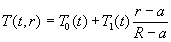 at a
≤ r ≤ R.
at a
≤ r ≤ R.
Here –T1
≤ T1(t) ≤ T1; min T0
≤ T0(t) ≤ max T0.
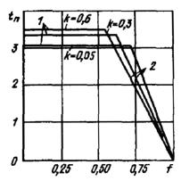
Fig. P4.38.
Diagrams of adaptability for a simply supported round plate with a force
distributed over the ring at T(t, r) = T0(t)
+ T1(t)(r – a)/(R –
a):
1 is an alternating flow;
2 is a progressive form change
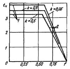
Fig. P4.39.
diagrams of adaptability for a simply supported round plate with a force
distributed over the ring at T(t, r) = T0(t)
+ T1(t)[(r – a)/(R –
a)]2:
1 is an alternating flow;
2 is a progressive form change
Loading parameters:
f = p*/(2pσsh2);
tp = t*/t0,
where t*
= αET1/[3(1 - k)σs]; t0 =
1.015; k = a/R.
Alternating
flow condition:
max[|φ(ρ)|,
|ψ(ρ)|, φ(ρ) - ψ(ρ)|]t* = 1;
φ(ρ) = ψ(ρ) =
1 - 1.5k + 0.5k2)(b - 2)/(b + k2)
at 0 ≤ ρ ≤ k;
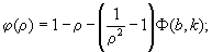
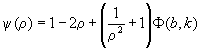 at k
≤ ρ ≤ 1.
at k
≤ ρ ≤ 1.
Here 

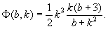
Progressive
form change condition:
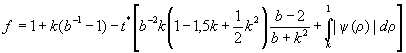
at x(k)
< 1;
 at x(k)
> 1.
at x(k)
> 1.
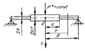
Fig. P4.40.
Simply supported round plate with a stepwise change in thickness
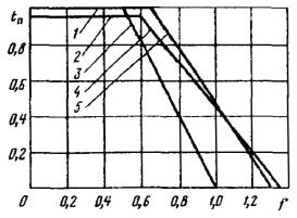
Fig. P4.41.
Diagrams of adaptability for a simply supported round plate with a step change
in thickness, loaded with a concentrated force:
1 is an alternating flow
for k = 0.25, b = 1; 2 is an alternating flow for k
= 0.25, b → 0; 3 is a progressive form change for k =
0.25, b = 1; 4 is a progressive form change for k = 0.25, b
→ 0; 5 is a progressive form change for k = 0.25, b = 2/3
Here 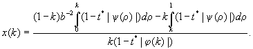
Fig. P4.41
shows diagrams of adaptability for a simply supported round plate with a step
change in thickness, loaded with a concentrated force.
7.16. For
cylindrical pipes loaded with inner pressure (or axial force) without bending
at cyclic temperature changes uniformly distributed along the pipe axis and
varying in thickness, the conditions for the start of form change (tolerance of
2 · 10-4%) and deformations accumulated over the cycle can be
determined in the range of operating temperatures up to 925 K (650 °C) at σRK/RTct
in Fig. P4.42 depending on σm/Rp0.2.
Here RTct is a creep limit at t = 2 · 105
h and accumulated plastic deformation limit 0.2 %; σRK is a
range of temperature stresses; σm is a pressure stress.
8. METHOD FOR DETERMINING
THE VALUE OF IRREVERSIBLE FORM CHANGE UNDER NEUTRON EXPOSURE CONDITIONS
8.1. The method
applies to the parts listed in item 5.8.
8.2. When
assessing the component of the value of irreversible form change from the
neutron radiation, the difference in the integral doses of exposure over the
part cross-section is not considered.
8.3. The
irreversible cumulative change in Δl size with neutron fluence Fn
shall not exceed the permissible irreversible size change of [Δl] and
neutron fluence [Fn] determined approximately in the range of
operating temperatures 623 - 923 K (350 - 650 °C) using the empirical formula
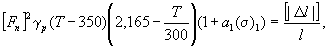
where T = Tmax,
°С; γp is a characteristic of the material swelling under
exposure by neutrons with an energy of more than 0.1 MeV (see Table P4.1);
(σ)1 is the highest reduced stress from mechanical load [(σ)1
< σs], MPa (kgf/mm2); a1 =
0.024 1/MPa (0.24 mm2/kgf).
8.4. Axial form
change under neutron exposure of parts with stationary axial temperature
gradients is determined by linear summation.
8.5. When
determining the value of irreversible form change under the conditions of joint
or separate action of thermal cycling and mechanical load and neutron
radiation, dimensional changes are linearly summed.
9. EXAMPLE OF
CALCULATING UPPER AND LOWER ESTIMATIONS OF LIMIT CYCLE PARAMETERS
9.1. This
example illustrates the procedure for calculating the upper and lower
assessments of parameters of the limit cycle using the general methods of the
theory of adaptability. The structure characteristics and loading conditions
are conditionally selected for the purpose of the most distinct presentation of
the calculation stages. Features of solutions under more difficult loading
conditions are considered at the end of each stage.
9.2. We
calculate the cylindrical shell clamped along the edges as shown in Fig. P4.43.
Inter alia, calculation of the shell, which has sufficiently rigid flanges at
the ends, whose temperature is equal to the temperature of the middle surface
of the shell, are reduced according to this scheme. The shell length l,
radius R, and thickness 2h are given. The shell is subjected to
the action of the constant inner pressure p and temperature T(t)
varying under linear law along the thickness of the shell at each moment of
time t:

Here T0(t)
is a middle surface temperature; T2(t) is a
temperature difference between the inner and outer surface of the shell.
Purpose of the
calculation is to determine the upper and lower assessments of the parameters
of the limit cycle and then compare them with the specified parameters of the
operating cycle in accordance with Section 5.4.
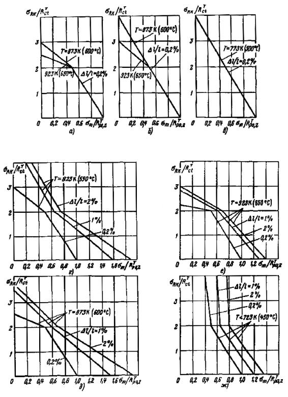
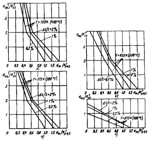
Fig. P4.42.
Diagrams of equal form change of components such as pipes (rods) at thermal
cycling and mechanical load after 1000 loading cycles with a duration of up to
2 · 105 h:
a are
nickel-chromium steels after cold-work hardening of up to 15%; b are nickel-chromium
precipitation-hardening steels; c, d, e, f are
nickel-chromium steels; g, h, i, j, k are
low-alloyed steels
9.3. When
calculating, the properties of the shell material (modulus of elasticity E,
temperature coefficient of linear expansion α, Poisson ratio μ, and limit
stresses σs) are determined in accordance with Section 6.3,
3.1 and 3.2 in the same way as was done in the previous example.
Numerical data are not given here, since in the calculation example below, it
is assumed that the value of σs is constant, and the
calculation of the upper and lower assessments is carried out in a general form
without using specific numerical values. Changes in the calculation procedure
when the numerical specification of variable σs are indicated
at the end of each calculation stage.
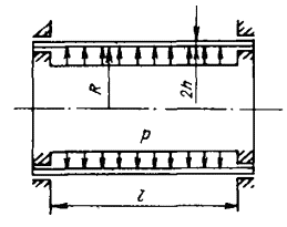
Fig. P4.43.
Shell design diagram
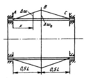
Fig. P4.44.
Distribution of increments of the shell radial displacements
Conditional
elastic stresses from uneven heating are determined by the formula
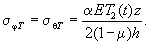
Here σφT,
σθT are circular and axial stresses, respectively; z
coordinate is measured from the middle surface of the shell along the normal to
it; z axis is directed to the shell axis, -h ≤ z ≤h.
9.4. Calculation
of the upper assessment of the progressive from change conditions.
Calculation is
held according to the following procedures:
a) in accordance with
item 5.6.8, the distribution of increments of radial displacements per
cycle Δw shown in Fig. P4.44 is set,
Δw = Δw02x/L
0 ≤ x ≤ L/2,
as well as zero
increments of axial displacements per cycle Δu
Δu =
0.
In accordance
with the diagram shown in Fig. P4.44, cross-sections A, B
and C have gaps in increments of axial displacements per cycle Δu'φ:
in cross-sections A and C Δu'φ = z2Δw0/L;
in cross-section В Δu'φ = -2zΔα = -z4Δw0/L;
b) using the
compatibility conditions of deformations, we find the increments of the
circumferential and axial deformations per cycle Δεθ, Δεφ
corresponding to the specified displacement increments at 0 < x <
0.5L.
For
cylindrical shell

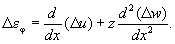
Substituting
the values of displacement increments here, we get
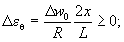 Δεφ
= 0;
Δεφ
= 0;
c) write the conditions:
existence of a progressive form change in accordance with item 5.6.5.
For the given
problem a = 1, b = 0, since Δε0 > 0, Δεφ
= 0. Provided that 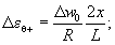 ; Δεφ+
= 0, since the increments of circumferential plastic deformations are positive;
; Δεφ+
= 0, since the increments of circumferential plastic deformations are positive;
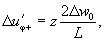 Δu'φ-
= 0 for cross-sections A and C at z > 0;
Δu'φ-
= 0 for cross-sections A and C at z > 0;
Δu'φ+
= 0,  for
cross-sections A and C at z < 0;
for
cross-sections A and C at z < 0;
Δu'φ+
= 0, 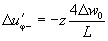 for
cross-section B at z > 0;
for
cross-section B at z > 0;
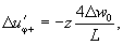 Δu'φ
= 0 for cross-section B at z < 0.
Δu'φ
= 0 for cross-section B at z < 0.
With due
regard to the symmetry of the distribution of plastic deformation increments
and the constancy of σs, σθT and σφT
values along the shell length, the condition for the existence of progressive
form change, given in item 5.6.5, takes the form of
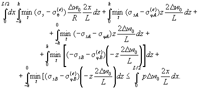 (P4.1)
Indices A
and B indicate that the corresponding values refer to cross-sections A
and B (see Fig. P4.44).
Let us find
the minimum values of the integrands of the left-hand side of this inequality
for the cycle time. Considering that
 x
> 0, Δw0 > 0,
x
> 0, Δw0 > 0,
and the values of conditional
elastic stresses σθ(e), σφ(e)
are determined in accordance with the expressions given in Sections 9.3
and 9.2, we get:
a) at –h ≤ z
≤ h
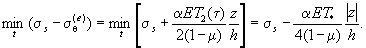
Note that at z>
0, the minimum is reached if T2(t) = T*/2,
and for z <0 - if 
b) at 0 ≤ z ≤ h
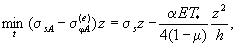
it is reached if 
c) at –h ≤ z
≤ 0
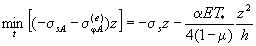
for 
d) at 0 ≤ z ≤h
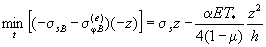
for
e) at –h ≤ z ≤ 0
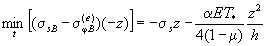
for 
Substituting
the obtained values into the inequality (P4.1), we obtain, after
integration, the condition for the progressive form change existence in the
form of
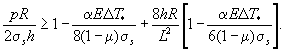 (P4.2)
Note that in
the general case, when the value of σs changes during a cycle
depending on temperature (and is variable along the shell volume), and the
temperature field of the shell is nonlinear and is set numerically, the
calculation sequence differs from the above one in that the integration in
inequality (P4.1) is carried out for the entire shell length (there is
no symmetry), and the minimum values of the integrands are found numerically by
comparing the corresponding values obtained for a number of moments in time.
The result
obtained is the upper assessment of the limit cycle parameters: it determines
the conditions of realization in the limit cycle of the field of increments of
displacements shown in Fig. P4.44.
9.5. Calculation
of the lower assessment of the progressive from change conditions.
In accordance
with item 5.6.2, the shell adaptability is ensured if it is possible to
specify time-independent stresses σθ0, σφ0,
satisfying:
a) equilibrium
conditions
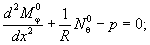 Nφ0 = 0; (P4.3)


 (P4.4)
(positive directions of
forces are shown in Fig. P4.45);
b) the inequality of
item 5.6.2, which, with due regard to item 5.6.3 with reference
to this problem, has the following form:
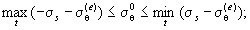
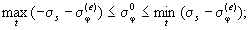
 .
.
Substituting
into this system the values of conditional elastic stresses (Section 9.3)
and taking into account the limits of temperature variation (Section 9.2),
at σs = const we obtain
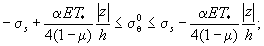 (P4.5)
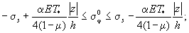 (P4.6)
-σs
≤ σθ0 - σφ0 ≤ σs.
(P4.7)
To obtain a
lower assessment of the conditions of adaptability, one shall set the values of
stresses σθ0, σφ0 so that
inequalities (P4.5) - (P4.7) are fulfilled, and find the corresponding
value p from conditions (P4.3) and (P4.4). To specify the
stresses σθ0, σφ0 we can use the
earlier introduced (when calculating the upper assessment of the conditions of
progressive form change) assumptions of the distribution of plastic deformation
increments (Fig. P4.44):
a) in accordance with
Fig. P4.44 everywhere in the shell, there is a tension in the
circumferential direction, so it can be assumed that the circumferential
stresses σθ0 everywhere reach the limit (upper) values
determined by inequalities (P4.5), that is
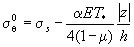 (P4.8)
(this stress
distribution is illustrated in Fig. P4.46, a);
b) symmetrical
distribution of displacement increments, shown in Fig. P4.44,
corresponds to the assumption of equality of bending moments at x = 0, x
= L:
(Mφ0)x=0
= (Mφ0)x=L;
c) suppose that the
axial stresses σφ0 are distributed over the shell
thickness according to a linear law (Fig. P4.46, b, c):
σφ0
= σφ*z/h.
The values of
σφ* may be different in different cross-sections of the
shell. Their numerical values are not specified yet. In the course of further
calculations, such σφ* values are found for which the
value of p is the greatest value when conditions (P4.3) - (P4.7)
are fulfilled. Note that the proposed law of stress distribution is not
directly related to the distribution of displacement increments, shown in Fig. P4.44;
d) transform the
constraint system (P4.3) - (P4.7) with due regard to assumptions
a), b) and c). Substituting the estimated values of the stresses in the
expression (P4.4), we get

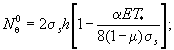 Na0
≡ 0.
Na0
≡ 0.
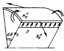
Fig. P4.45.
Positive directions of forces
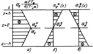
Fig. P4.46.
Assumed distribution of stresses
Substitute the
obtained values of the forces in the equilibrium equation (P4.3). After
double integration, with due regard to the assumed equality of the bending
moments at x = 0 and x = L, this equation takes the form
of
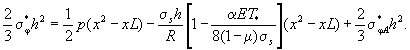 (P4.9)
Inequalities (P4.5)
are satisfied everywhere in the shell in accordance with assumption a). To
fulfill the inequalities (P4.6), (P4.7) at all points of any
cross-section of the shell, it is sufficient that they are fulfilled at z
= h and z = -h (since, with due regard to the assumed
distributions of stresses σφ* and σθ*,
the left and right sides of each of these inequalities contain linear functions
of the z coordinate and, moreover, σφ0 = 0 at z
= 0). In this case, conditions (P4.6) have the following form:
 (P4.10)
and conditions (P4.7)
have this form:
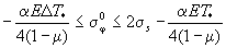 at z
= h and z = -h.
at z
= h and z = -h.
This
inequality is transformed with due regard to the relations
σφ0
= σφ* at z = h and σφ0
= -σφ* at z = -h
to the following:
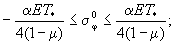 (P4.11)
e) to satisfy the
inequalities (P4.10), (P4.11) in all cross-sections of the shell,
it is enough that they are fulfilled where the stresses σφ*
reach extreme (greatest and smallest) values. In accordance with the equation (P4.9)
such values can be achieved at the edges of the shell (at x = 0 and x
= L; stresses σφ* = σφA*)
or at x = 0.5L, since in this cross-section
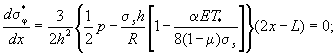
provided that
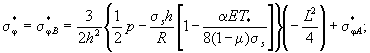
f) according to the last
equation we find the pressure p:
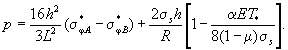
Substituting
here the values of stresses σ*φA, σ*φB,
satisfying inequalities (P4.10) and (P4.11), we obtain the
pressure value p, which is the lower assessment of the adaptability
conditions. The best assessment obtained in this way has the form of
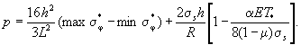 (P4.12)
The greatest
value of stresses σφ*, at which all inequalities (P4.10)
and (P4.11) are satisfied, is equal to
 if
if 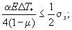
 if
if 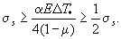
The smallest
value of stresses σφ*, at which inequalities (P4.10)
and (P4.11) are satisfied, is equal to
 if
if
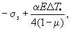 if
if 
Substituting
these values into equation (P4.12), we find that the shell adaptability
is guaranteed if
 at
at  (P4.13)
at
 (P4.14)
These results
illustrate at L2/(8Rh) = 0.6 lines 2 and 3
in Fig. P4.47; here, the upper assessment of the conditions of
progressive form change (P4.2) corresponds to line 1.
Note that in
the general case, when the σs values change during a cycle
depending on temperature, and the temperature field of the shell is nonlinear
and numerically specified, the calculation sequence differs from the one given
above in that:
a) when obtaining the
equation (P4.9) from the equilibrium conditions (P4.3), the
integration of the circumferential forces Nθ0 is
carried out numerically;
b) location of the
cross-sections in which the stresses σφ* reach extreme
values, as well as the values of stresses σφ* ensuring
the fulfillment of constraints - inequalities, are determined by selection.
9.6. Comparison
of the upper and lower assessments of the parameters of the limit cycle with
the parameters of the operating cycle. Refinement of the upper and lower
assessments.
After
obtaining the upper and lower assessments of the parameters of the limit cycle
they are compared with the parameters of the operating cycle in accordance with
Section 5.4.
If the
parameters of the operating cycle are higher than the upper assessment of the
parameters of the limit cycle, then adaptability is impossible.
If the
parameters of the operating cycle are lower than the lower assessment of the
parameters of the limit cycle, then the structure will adapt to the given
impacts.
If the
parameters of the operating cycle are lower than the upper, but higher than the
lower assessment of the parameters of the limit cycle (this is possible with a
significant difference between the upper and lower assessments), then a refined
calculation of the parameters of the limit cycle is performed.
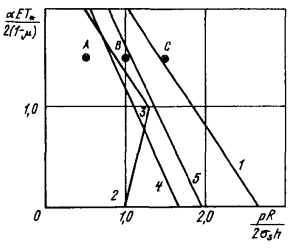
Fig. P4.47.
Shell adaptability diagram
Consider three
examples of calculations that differ in a given pressure in the operating cycle
with the same geometrical characteristics of shell [L2/(8Rh)
= 0.6] and the same temperatures (αEΔT/[2(1 - μ)] = 1.5). Let for
given operating conditions of the shell
a)  b)
b)
 c)
c)

The specified
values of the parameters of the operating cycle correspond to points A, B
and C in Fig. P4.47. In accordance with condition (P4.2),
adaptability for the case under consideration is impossible if

Hence, at pR/(2σsh)
= 1.5 the adaptability is impossible.
In accordance
with condition (14) of Section 9.5, adaptability is provided if pR/(2σsh)
<0.9. Hence, at pR/(2σsh) = 0.5 the shell will
adapt to the given impacts.
Finally, at pR/(2σsh)
= 1, the obtained upper and lower assessments do not allow us to answer the
question about the possibility of adaptability. Note that when calculating in
Section 9.5 the revised lower assessment, the distribution of
circumferential stresses was assumed as it really is in the limit cycle if
there is no bending. Therefore, the lower assessment obtained above in the
limit (at L → ∞) coincided with the upper assessment, but
for short shells, in the form change of which the bending plays a significant
role, this lower assessment is far from the exact solution. To get the best
lower assessment for short shells, we set
σθ0
= 0; 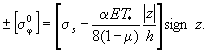
In one
cross-section, only the upper or only lower sign is used.
A solution
similar to that discussed in Section 9.5, then leads to the following
condition of adaptability:
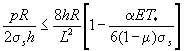
(it corresponds to line
4 in Fig. P4.47).
Comparison of
this result with the upper assessment (2) shows that the difference between
them decreases with decreasing value of L2/(8Rh) and
becomes negligible for sufficiently short shells. However, at
 and
and 
the lower assessment
obtained here gives pR/(2σsh) ≤ 0.83, i.e. it turns
out to be worse than the lower assessment obtained in Section 9.5.
To improve the
lower assessment for shells of average length, non-zero circumferential
stresses σθ0 should be specified which provide for
obtaining larger bending moments Mφ0 than those
obtained in Section 9.5. Let, for example,
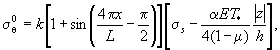
where k is an
unknown factor which is selected during the solution so as to obtain the best
lower assessment 0 ≤ k ≤ 0.5. Result of the calculation similar to that
discussed in Section 9.5 is shown by the line 5 in Fig. P4.47 at
αET*/[2(1 - μ)] = 1.5; the appropriate condition of
adaptability has the form of

Thus, at pR/(2σsh)
= 1, the will be no progressive form change of the shell.
APPENDIX 5
(recommended)
CALCULATION OF TYPICAL ASSEMBLIES OF
PARTS AND STRUCTURES
1. BASIC PROVISIONS
This Appendix
contains recommended methods for determining the stresses in pipelines and
detached connections of vessels.
Selection of
the basic dimensions of the components of structures (wall thickness) is
carried out according to the formulas of Section 3 hereof.
The
calculation is performed for operation modes and for the main design loads
indicated in items 5.1.3, 5.1.4 of the Regulations.
The formulas
for calculating stresses given in this Appendix do not exclude the possibility
of using more accurate formulas and relations for the calculation of
structures.
2. PIPELINES
2.1. CONVENTION SYMBOLS
Da is an nominal outer diameter of the
pipe, mm
D is an inner diameter (D = Da
– 2s), mm
s is a nominal
wall thickness of the pipe, mm
r is a mean
radius of the cross-section [r = (Da - s)/2],
mm
R is a radius of curvilinear pipe axis, mm
a is an
ellipticity (out-of-roundness) of the cross-section (the ratio of the
difference between the maximum and minimum outer diameters of the cross-section
to their half-sum),%
As is a pipe
cross-sectional area, mm2
W is a moment of resistance to the pipe
cross-section bending, mm3
λ is a dimensionless
geometric parameter (λ = Rs/r2)
p is a design
inner pressure in the pipeline, MPa
Mx, My, Mz
are bending and torque moments in the pipeline cross-section, N · mm
Nz is an axial force in
the cross-section of the pipeline from the action of a mass load and
self-compensation of temperature expansions, N
ω is a dimensionless
parameter of inner pressure 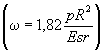
E is a modulus of elasticity of the material, MPa
Kp is a coefficient of
compliance of a curvilinear pipe, taking into account the effect of inner
pressure (the ratio of compliances to the bending of curvilinear and
rectilinear pipes of the same cross-section and made of the same material)
K*p is a
coefficient of compliance of a curvilinear pipe, taking into account the effect
of inner pressure and interface with rectilinear pipes
γm is
a coefficient of intensification of bending transverse stresses in a
curvilinear pipe.
βm is
a coefficient of intensification of bending longitudinal stresses in a
curvilinear pipe
σ0zMN,
σ0zMN(s) are longitudinal
stresses due to bending moment and axial force, MPa
σψ is a
circumferential (tangential) stress in a pipe wall, MPa
σz is
an axial (longitudinal) stress in a pipe wall, MPa
σr is
a radial stress in a pipe wall, MPa
τ is a torsional stress,
MPa
σTp, σT0,
σT are temperature stresses, MPa
(σ)2, (σ)RK,(
σaF)K, (σ)p are reduced
stresses, MPa
[σ] is a nominal
permissible stress, MPa
φw –
coefficient of strength reduction of a weld seam
ασ is a
tangential stress concentration coefficient
Ki(s) is a coefficient of
local bending stresses in the pipe from the impact of the nozzle.
2.2. GENERAL
2.2.1. This
Section covers the calculation of low-temperature and high-temperature NNP
pipelines. The class of low-temperature pipelines includes pipelines made of
carbon, alloyed, silicon-manganese and high-chromium steels, of austenitic
steels, heat-resistant chromium-molybdenum-vanadium steels, iron-nickel alloys
and zirconium alloys with a design temperature of not more than Tt.
The class of high-temperature pipelines includes pipelines with a higher design
temperature exceeding temperature Tt (item 3.2
hereof).
2.2.2. When
determining the reduced stresses of different categories, the loads shall be
considered according to item 5.1.3 hereof.
2.2.3. Internal
forces in the pipeline are determined with due regard to all influencing
factors, inter alia, with due regard to the friction forces arising in the
sliding supports, as well as the suspension deviation from the vertical
position.
2.2.4. Presence of
two signs (plus, minus) in front of the additive in the formulas given means
that the calculation of the reduced stresses using this formula is performed
both when the plus sign is accepted and when the minus sign is accepted. To
assess the strength, a larger value of the reduced stress is taken.
2.2.5. The reduced
rigidity of the curvilinear segment for bending is taken into account in the
calculation by introducing the coefficient of compliance for it. The latter
takes into account the deformation (flattening) of the cross-section and is
determined according to Section 2.5.
2.2.6. It is
allowed to determine stresses in a curvilinear pipe by the procedure of Section
2.8.
2.2.7. It is
allowed to determine stresses in a tee connection by the procedure of Section 2.9.
2.3. LOW-TEMPERATURE PIPELINES
2.3.1.
Determination of stresses (σ)2.
2.3.1.1. For
rectilinear and curvilinear pipes, the stress state components are determined
by the formulas
σψ
= σψp,
where 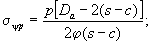
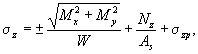
where 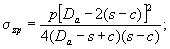
σr
= -p/2; 
The value of
the strength reduction coefficient φ is assumed in accordance with item 4.3
of the Regulations.
The force Nz
is considered positive if it causes pipe stretching.
2.3.1.2. For
curvilinear pipes, the geometrical parameter λ of which satisfies the condition
λ ≤ 1.4, in addition to determining the reduced stress (σ) 2, using
the formulas in item 2.3.1.1, the reduced stress is calculated by the
formula
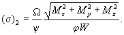
The values of
Ω and ψ are determined by Tables P5.1 and P5.2 applying a linear
interpolation method.
2.3.1.3. For the tee
assembly, the stress (σ) 2 is calculated for three cross-sections: A-A,
B-B, C-C (Fig. P5.1). Below are the formulas
for calculating the components of the stress state:
Table P5.1.
Value of coefficient ψ
|
ψ
|
1.0
|
0.98
|
0.94
|
0.88
|
0.79
|
0.68
|
0.50
|
0.30
|
0.10
|
|
σψp/[σ]
|
0
|
0.2
|
0.4
|
0.6
|
0.8
|
1.0
|
1.2
|
1.4
|
1.6
|
Table P5.2.
Value of coefficient Ω
|
Ω
|
18
|
10
|
6
|
3
|
2
|
1.7
|
1.0
|
0.65
|
|
λ
|
0
|
0.05
|
0.1
|
0.2
|
0.3
|
0.4
|
0.9
|
1.6
|
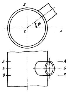
Fig. P5.1. Tee
assembly (pipe with nozzles)
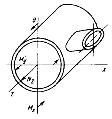
Fig. P5.2.
Force factors in the cross-section of the tee assembly
for cross-sections A-A
and C-C
σψ
= σψp;
σz
= σ0zMN ± 0.7σ0zMN(s)Ki(s)
+ σzp;
for cross-section B-B
σψ
= σψp ± 0.7σ0zMN(s)Ki(s);
σz
= σ0zMN + σzp.
Stresses τ, σψp,
σzp, σr in these cross-sections are
determined by the formulas of item 2.3.1.1. The longitudinal stress in
the pipe is determined by the formula
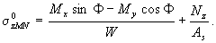
Force factors Mx,
My, Nz considered positive if directed as
shown in Fig. P5.2. Angle Φ determines the nozzles position (Fig. P5.1).
The
longitudinal stress in the nozzle is calculated by the formula
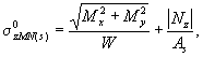
where the formula
quantities refer to the cross-section of the nozzle at the point of connection
with the pipe.
Coefficient of
local stresses Ki(s) is determined according to
Section 2.7.
2.3.2.
Determination of stress (σ)RK.
2.3.2.1. For
rectilinear and curvilinear tubes with λ ≥ 1.4, the stress state components for
the outer surface are determined by the formulas
σψ
= 2σzp;
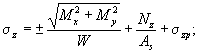
σr
= 0; τ = Mz/(2W).
2.3.2.2. For
curvilinear pipes with λ <1.4, the stress (σ)0RK
is determined by the following four formulas:
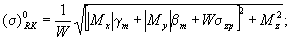
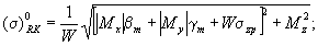
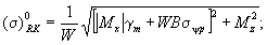
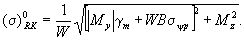
To assess the
strength, the larger of the four values is taken.
Coefficients γm
and βm are determined by Section 2.6. Stresses σzp
and σψp are determined by the formulas in item 2.3.1.1.
Coefficient B is calculated by the formula

2.3.2.3. For the
tee assembly, the stresses are calculated using the formulas:
for cross-sections A-A
and C-C (Fig. P5.1)
σψ
= 0.5ασσψp;
σz
= σ0zMN ± σ0zMN(s)Ki(s)
+ σzp;
for cross-section B-B
σψ
= σψз ± σ0zMN(s)Ki(s);
σz
= 1.5σ0zMN + σzp.
Radial stress
is assumed as σr = 0. Values of σψp, σzp,
σ0zMN, σ0zMN(s),
τ are calculated by the same formulas as in item 2.3.1.3, but at
φ = 1. For determining Ki(s) - see Section 2.7.
Coefficient of
concentration of tangential stresses at the edge of the hole ασ is
determined by the formula
ασ
= 1.2[2 + 2(D/Da)2 - (D/Da)4].
2.3.2.4. In the
places of conjugation of components with different wall thicknesses or with
different thermal and physical characteristics, the range of common temperature
stresses due to axial temperature difference (stress (σ)T0
are considered.
Stress (σ)T0
is determined by the formula
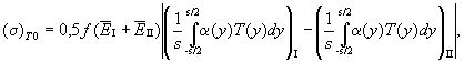
where y is a
distance from the middle of the wall according to normal; T(y) is
a wall temperature; α(y) is a coefficient of linear expansion of the
wall material;  is a
mean thickness modulus of elasticity.
is a
mean thickness modulus of elasticity.
Indices I and
II are used to denote mating components.
The wall
thickness shall be taken as maximum within the distance  from the
cross-section separating components I and II. Value of the coefficient f
is determined by linear interpolation according to the following values of
Table P5.3.
from the
cross-section separating components I and II. Value of the coefficient f
is determined by linear interpolation according to the following values of
Table P5.3.
2.3.2.5. Range of
the stress (σ)RK is determined by summing:
(σ)RK
= (σ)0RK + (σ)T0,
where (σ)0RK
is a range of reduced stress, calculated without taking into account the
temperature components of the uneven temperature field in the wall.
2.3.3.
Determination of stresses (σaF)K.
2.3.3.1. For
rectilinear and curvilinear tubes with λ > 1.0, the stress state components
(amplitude values) are determined by the formulas
σψ
= σzp;
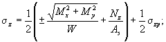
τ = Mz/(4W);
σr = 0.
Table P5.3. Values
of coefficients f
|
sI/sII
|
0
|
0.2
|
0.4
|
0.6
|
0.8
|
1.0
|
|
f
|
1.80
|
1.35
|
0.71
|
0.35
|
0.15
|
0
|
For the
formula determining σzp see item 2.3.1.1.
2.3.3.2. For
curvilinear pipes, the stress  is calculated by the
formulas
is calculated by the
formulas
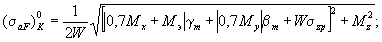
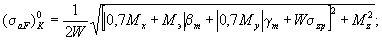

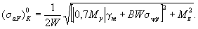
To assess the
strength, the larger of the four values is taken. The value of Me
is determined by the formula
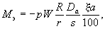
where x is a coefficient
taking into account the difference between the actual shape of the
cross-section distortion from the ideally elliptical. It shall be assumed that
x = 2.0.
Positive
direction of the bending moments is shown in Fig. P5.3.
Coefficients γm
and βm are determined by Section 2.6. Stresses σzp,
σψp are calculated by the formulas in item 2.3.1.1.
Coefficient B is determined according to item 2.3.2.2.
2.3.3.3. For the tee
assembly, determine the components of the stress state (amplitude values) by
the following formulas:
for cross-sections A-A
and C-C (see Fig. P5.1)
σψ
= 0.35ασσψp;
σz
= (1/2)[σ0zMN ± σ0zMN(s)Ki(s)
+ σzp];
for cross-sections B-B
σψ
= (1/2)(σψF ± σ0zMN(s)Ki(s));
σz
= (1/2)(3σ0zMN + σzp].
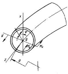
Fig. P5.3.
Positive directions of bending moments in a cross-section of a curvilinear pipe
Torsion stress
τ is determined by the formula in item 2.3.1.1, but with a
decrease of 2 times. Radial stress σr = 0. Values of σψp,
σzp, σ0zMN, σ0zMN(s),
Ki(s), ασ are determined in the same way as
required under item 2.3.2.3.
2.3.3.4. The range
of the total maximum temperature stress from the temperature difference across
the wall thickness [stress (σ)*T] and stress (σ)T0
from the axial temperature difference are determined. Calculation of (σ)*T
is carried out by analytical or numerical procedure, and calculation of (σ)T0
– by the formula in item 2.3.2.4.
2.3.3.5. Stress (σaF)K
for the loading cycle of each type is allowed to be determined by summing by
the formula
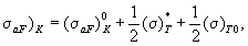
where (σaF)0K
is an amplitude of reduced stress, calculated without taking into account the
temperature components of the uneven temperature field in the wall.
2.3.4. Strength
criteria.
Strength
verification for stress categories (σ)2, (σ)RK is
carried out according to Section 5.4 hereof. Strength verification for
stress categories (σaF)K is carried out
according to Section 5.6 hereof.
2.4. HIGH-TEMPERATURE PIPELINES
2.4.1.
Determination of stresses (σ)2, (σ)RK, (σaF)K.
2.4.1.1. When
determining the reduced stress (σ)2, the axial stress σz
is calculated with due regard to the strength reduction coefficient of the
transverse weld by the formula
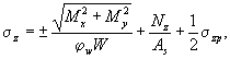
where the strength
reduction coefficient φw is determined according to the
instructions of item 4.3.3 hereof.
As for the
rest, the reduced stresses (σ)2, (σaF)K
are determined by the same formulas that are used in the calculation of the
low-temperature pipeline (see items 2.3.1, 2.3.2, 2.3.3).
2.4.2.
Determination of stress (σ)RK.
2.4.2.1. In addition
to the given reduced stresses, reduced stress (σ)RK is
determined to evaluate the long-term static strength with due regard to local
stresses and action of all loads (pressure, mass load, compensation) it a
steady-state operation mode. In this case, the components of the stress state
due to the compensation of temperature expansions are allowed to be determined
with due regard to the gradual decrease (relaxation) in time due to creep.
2.4.2.2. Components
of the stress state for rectilinear pipes and curvilinear pipes with λ ≥ 1.0
are determined by the formulas in item 2.3.1.1.
2.4.2.3. For
curvilinear pipes (at any value of λ), the stress (σ)RK is
calculated by the following formulas:
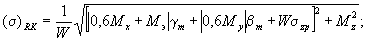
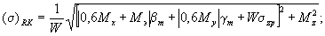
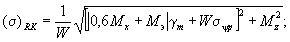
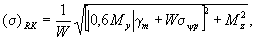
where 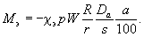
The value of χe
is determined by linear interpolation according to Table P5.4.
Table P5.4. Value
of coefficient χe
|
Steel
|
Temperature,
°С
|
|
360
|
450
|
500
|
550
|
600
|
650
|
700
|
|
Carbon and
silicon-manganese
|
0.4
|
0.35
|
-
|
-
|
-
|
-
|
-
|
|
Chrome-molybdenum and
chrome-molybdenum-vanadium
|
0.5
|
0.45
|
0.4
|
0.35
|
0.2
|
-
|
-
|
|
Austenitic
|
-
|
0.55
|
0.5
|
0.4
|
0.35
|
0.3
|
0.2
|
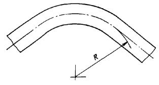
Fig. P5.4.
Curvilinear pipe
Stresses σzp
and σψp are determined by the formula in item 2.3.1.1,
coefficients γm, βm – by the Section 2.6.
2.4.2.4. For the tee
assembly, components of the stress state are determined by the formulas:
σψ
= 1.5σψp;
σz
= σ0zMN ± σ0zMN(s)Ki(s)
+ σzp,
for cross-section B-B
σψ
= σψp ± σ0zMN(s)Ki(s);
σz
= 1.5σ0zMN + σzp.
Values of σzp,
σψp, σ0zMN, σ0zMN(s),
τ are determined in the same way as required under item 2.3.2.1.
Value of Ki(s) is calculated according to Section 2.7.
2.4.3. Strength
criteria.
2.4.3.1. Strength
verification for stress categories (σ)2 and (σ)RK
is carried out according to Section 5.4 hereof, and for category (σaF)K
– according to Section 5.6 hereof.
2.5. DETERMINATION OF THE COMPLIANCE COEFFICIENT OF
THE CURVILINEAR PIPE
2.5.1. The
compliance coefficient of curvilinear pipe (Fig. P5.4) is calculated as
the product of the compliance coefficient Kp, determined
without taking into account the constraint of deformation of its ends from the
influence of adjacent pipes on the coefficient ζ, taking into account this
constraint of deformation, i.e.
K*p = ζKp.
Table P5.5. Value
of coefficient ζ
|
λ
|
The angle
between the end sections of the pipe, deg
|
|
0
|
30
|
60
|
90
|
|
R/r
|
R/r
|
R/r
|
R/r
|
|
2
|
4
|
6
|
8
|
2
|
4
|
6
|
8
|
2
|
4
|
6
|
8
|
2
|
4
|
6
|
8
|
|
0
|
0.0
|
0.0
|
0.0
|
0.0
|
0.12
|
0.18
|
0.24
|
0.28
|
0.25
|
0.37
|
0.47
|
0.55
|
0.42
|
0.58
|
0.65
|
0.70
|
|
0.2
|
0.12
|
0.12
|
0.12
|
0.12
|
0.27
|
0.34
|
0.39
|
0.42
|
0.43
|
0.56
|
0.66
|
0.73
|
0.60
|
0.78
|
0.84
|
0.88
|
|
0.4
|
0.24
|
0.24
|
0.24
|
0.24
|
0.43
|
0.48
|
0.52
|
0.54
|
0.62
|
0.73
|
0.80
|
0.84
|
0.77
|
0.88
|
0.91
|
0.93
|
|
0.6
|
0.37
|
0.37
|
0.37
|
0.37
|
0.55
|
0.59
|
0.61
|
0.62
|
0.73
|
0.81
|
0.85
|
0.88
|
0.82
|
0.90
|
0.94
|
0.95
|
|
0.8
|
0.49
|
0.49
|
0.49
|
0.49
|
0.63
|
0.66
|
0.68
|
0.69
|
0.77
|
0.84
|
0.88
|
0.90
|
0.85
|
0.92
|
0.93
|
0.94
|
|
1.0
|
0.60
|
0.60
|
0.60
|
0.60
|
0.72
|
0.74
|
0.75
|
0.76
|
0.83
|
0.88
|
0.91
|
0.93
|
0.89
|
0.94
|
0.96
|
0.96
|
|
1.2
|
0.73
|
0.73
|
0.73
|
0.73
|
0.80
|
0.82
|
0.83
|
0.84
|
0.88
|
0.91
|
0.94
|
0.95
|
0.92
|
0.95
|
0.97
|
0.97
|
|
1.4
|
0.85
|
0.85
|
0.85
|
0.85
|
0.89
|
0.90
|
0.91
|
0.91
|
0.93
|
0.95
|
0.96
|
0.96
|
0.96
|
0.97
|
0.98
|
0.98
|
|
1.65
|
1.00
|
1.00
|
1.00
|
1.00
|
1.00
|
1.00
|
1.00
|
1.00
|
1.00
|
1.00
|
1.00
|
1.00
|
1.00
|
1.00
|
1.00
|
1.00
|
2.5.2. Compliance
coefficient Kp is determined by the formula
Kp = 1 + 1.125/b.
The value of b
is calculated by the following formulas:
a1 = 1.0100 +
1633.5λ2 + 99.00ω;
a = 1.0156 +
661.5λ2 + 63.00ω – 0.2316/a1;
a3 = 1.0278 +
204.2λ2 + 35.00ω – 0.2197/a2;
a4 = 1.0625 +
37.5λ2 + 15.00ω – 0.1914/a3;
b = 0.1250 +
1.5λ2 + 3.00ω – 0.09766/a4.
λ and ω
parameters are calculated by the formulas


2.5.3. ζ
coefficient is determined by the method of linear interpolation according to
data in Table P5.5.
2.6.
DETERMINATION OF COEFFICIENTS OF STRESS INTENSIFICATION FOR THE CURVILINEAR
PINE
2.6.1. Stress
intensification coefficient γm and βm are determined
by the formulas
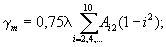
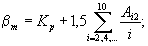
where A22
= -1/b; 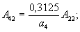
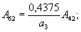
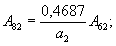
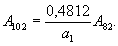
Values of Kp,
a1, a2, a3, a4,
b are determined by the formulas in Section 2.5.
2.7. DETERMINATION OF THE COEFFICIENT OF LOCAL
BENDING STRESSES FOR THE TEE ASSEMBLY
2.7.1. At  (Fig. P5.5)
coefficient of local stresses Ki(s) is calculated by
the formula
(Fig. P5.5)
coefficient of local stresses Ki(s) is calculated by
the formula
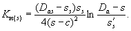
Size s's
is determined by Fig. P5.5.
2.7.2. When 

2.7.3. If the
value of Ki(s), calculated by the formula in item 2.7.1
or 2.7.2, is less than 2, it shall be assumed that Ki(s)
= 2.
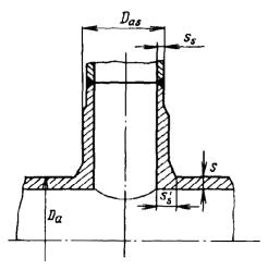
Fig. P5.5. Tee
assembly
2.8. CALCULATION OF STRESSES IN A CURVILINEAR PIPE
BY REFINED PROCEDURE
2.8.1. Circular
section pipe.
2.8.1.1. Calculate
the normal stresses from bending of the pipe without taking into account
deformation of the cross-section:
σ0az(x)
= Mx/W; σ0az(y)
= My/W;
σ0z(x) = σ0az/β; σ0az(y) = σ0az(y)/β,
where β = Da/D.
Hereinafter, the index a denotes the outer surface. (For the direction
of moments, see Fig. P5.3.)
2.8.1.2. The
stresses caused by torque, inner pressure, and axial force, are calculated:
τa
= Mz/(2W); τ = τa/β;
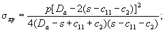
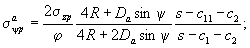
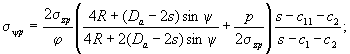
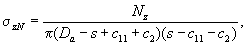
where s is a
minimum wall thickness due to process operations; φ – see item 2.3.1.1;
ψ – see Fig. P5.3.
2.8.1.3. Calculate
the bending stresses with due regard to deformation of the cross-section:
σazM
= σ0az(x)βa1
+ σ0az(y)βa2;
σzM = σ0z(x)β1 + σ0z(y)β2;
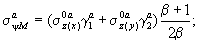
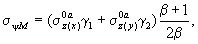
where
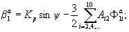
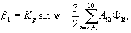

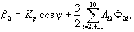
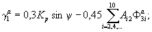
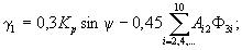
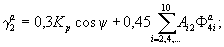
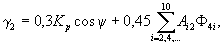
provided that (replace i
and j with one letter v for short)
Φ1v = sin ψ
cos vψ – (1/v)cos ψ sin vψ ± 0.15λ(1
– v2)cos vψ;
Φ2v = sin ψ
sin vψ + (1/v)cos ψ cos vψ ± 0.15λ(1
– v2)sin vψ;
Φ3v = sin ψ
cos vψ – (1/v)cos ψ sin vψ ±
(λ/0.6)(1 – v2)cos vψ;
Φ4v = sin ψ
sin vψ + (1/v)cos ψ cos vψ ±
(λ/0.6)(1 – v2)sin vψ;
where the upper sign
corresponds to the inner surface, and the lower sign – to the outer.
Values of Kp
and Ai2 are determined according to items 2.5.2
and 2.6.1.
2.8.1.4. Calculate
the tangential membrane stresses from the bend of the pipe:
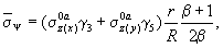
where 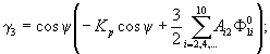
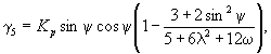
provided that
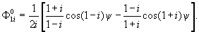
2.8.1.5. Calculate
the total normal stress on mutually perpendicular areas:
σaz
= σazM + σzN + σzp;
σaψ = σaψM +  + σaψp;
σz
= σzM + σzN + σzp; σψ
= σψM +  + σψp.
2.8.1.6. The reduced
stresses on the inner and outer surfaces of the pipe are determined for the
following sequence of values of the angle ψ: ψn = nhψ,
n = 0, 1, 2, ..., 35, where is the angle change pitch hψ
= 2p/36.
Radial normal
stress for the inner surface σr = -p, and for the
outer surface σar = 0.
2.8.2. Oval
section pipe.
2.8.2.1. It is
assumed that the cross-section of the pipe has an elliptical (oval) shape, with
the major axis of the cross-section perpendicular to the plane of the pipe
axis. The radial deviations of the contour of such a cross-section from a
circle of radius r are expressed by the equation (Fig. P5.3)
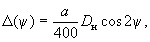
where a is an
out-of-roundness of cross-section (a ≤ 10 %).
2.8.2.2. Calculate
the normal stresses due to the initial out-of-roundness of the cross-section
for the inner and outer surfaces:
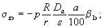
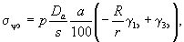
where β1e = β1
- sinψ; γ1e = γ1 - 0.3sinψ; γ3e = -γ3
- cos2ψ.
Determination
of β1, γ1 for inner and outer surfaces – see item 2.8.1.3,
and determination of γ3 – see item 2.8.1.4.
2.8.2.3. To take
into account the stresses determined according to item 2.8.2.2, they are
summed with the stresses of item 2.8.1.5, and then the reduced stresses
are determined at the points specified in item 2.8.1.6.
2.8.3. Features of
the calculation of stresses of various categories.
2.8.3.1. In
determining the stresses of categories (σ)RK and (σaF)K
for low-temperature pipelines, it is assumed that φ = 1. When calculating the
reduced stresses of category (σaF)K bending
stresses determined according to item 2.8.1.3 are multiplied by a coefficient
of 0.7. When calculating the stresses of category (σ)RK for
high-temperature pipelines, the value of the coefficient φ is assumed according
to Section 4.3 hereof, bending stresses of item 2.8.1.3 are
multiplied by a coefficient of 0.6, and bending stresses of item 2.8.2.2
are multiplied by a coefficient χe, where χe value is
assumed according to item 2.4.2.3.
2.9. CALCULATION OF STRESSES IN A TEE CONNECTION BY
REFINED PROCEDURE
2.9.1. For tee
connections of low-temperature pipelines formed by the intersection of two
circular cylindrical shells of constant thickness (nozzles and pipes with
diameters of the middle surface dm, Dm and
thicknesses ss, s) whose axes intersect at a right
angle, the refined calculation of the stress state is carried out for the
combined effect of inner pressure and significant loads in the end sections of
the tee: axial forces, bending and torque moments (Fig. P5.6, P5.7).
The procedure is applicable to compounds close to those mentioned in
geometrical form, covers the range of tees from thin-walled (ss/dm,
s/Dm = 0.01) to thick-walled (ss/dm,
s/Dm = 0.15), from equal (Dm/dm
= 1) to essentially unequal (Dm/dm >>
1), from having equal walls (ss = s) to having
different ones (s = 2ssDm/dm),
including "equal in strength" (ss/dm
= s/Dm). The actual geometry of the weld when
calculating the welded tee is not taken into account (in the margin of safety).
2.9.2. The input
data for the calculation of stresses in the tee are the following values (in
the agreed units of measurement, Fig. P5.6, P5.7): ss
is a wall thickness of the outlet (nozzle); s is a wall thickness of the
pipe (body); dm is a diameter of the middle surface of the
outlet (dm = 2rm = da –
ss); Dm is a diameter of the middle surface
of the pipe (Dm = 2Rm = Da
- s); p is an inner pressure; Nz3, Mx3,
My3, Mz3 are loads in the
cross-section of the outlet 3-3 axial force, bending moment in the plane of the
tee, bending moment from the plane of the tee, torque; Nzα,
Mxα Myα, Mzα
are axial force, moment in the plane of the tee, moment from the plane of the
tee, and torque in cross-sections of the pipe 1-1 (α = 1) and 2-2 (α = 2).
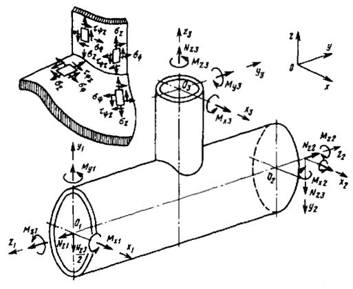
Fig. P5.6.
Positive directions of force factors
Force factors Nzi,
Mxi, Mii, Mzi (i =
1, 2, 3), positive directions of which are shown in Fig. P5.6, are
determined for the corresponding cross-sections (Fig. P5.7) from the
calculation of the pipeline system and satisfy the equilibrium conditions:
Mx1 + Mx2
+ Mx3 = 0;
My1 – My2
+ Mz3 = 0;
Mz1 – Mx2
– My3 = 0.
Self-balanced
loads in the end sections of the pipe (1-1 and 2-2), appearing in the formulas
of item 2.9.3 of the procedure, are calculated as follows:
Nz = (Nz1
+ Nz2)/2;
Mx = (Mx1
– Mx2)/2;
My = (My1
+ My2)/2;
Mz = (Mz1
+ Mz2)/2.
Fig. P5.7.
Design cross-sections of tee connection
2.9.3. Below are
the formulas and nomograms for calculating the components of the stress state σψ,
σz, σr and τ (their orientation is
shown in Fig. P5.6) in three cross-sections of the tee, determining its
strength. For equal and similar tees (Dm/dm
< 1.3), the calculation is carried out using additional formulas that take
into account the peculiarities of the distribution of stresses in this class of
tees. To assess the strength, the greater of the obtained values of the reduced
stresses are taken.
2.9.3.1. Stress
state components σψ and σz for stress group (σ)2
are determined by the following formulas:
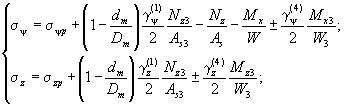
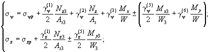
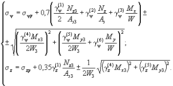
At ratio Dm/dm
< 1.3, the following stresses are additionally calculated:
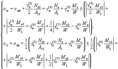
Radial
stresses σr are assumed as
σr
= -0.5p;
shear stresses τ are determined
by the formula
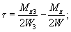
σψp
and σzp are calculated by the formula in item 2.3.1.1
(Da = D + s); As and As3
are cross-sectional areas of the pipe and nozzle; W and W3
are corresponding moments of resistance. Local stress coefficients γψ(i)
and γz(i) (i = 1, 2, ..., 8) are
determined according to item 2.9.3.4, force factors in the pipe Nz,
Mx, My, Mz are determined
by the formulas in item 2.9.2 from mass and other mechanical loads.
2.9.3.2. Components
of the stress group (σ)RK are calculated using the following
formulas (from pressure, mechanical and temperature effects):
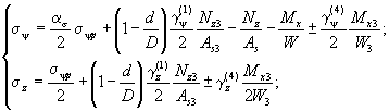
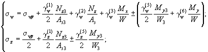
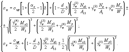
At Dm/dm
< 1.3, stresses are additionally determined:
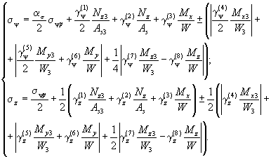
Radial
stresses σr = 0; torsion stress is determined by the formula
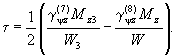
Coefficients
of local stresses γψ(i), γz(i),
γψz(i) (i = 1, 2, ..., 8) are found
according to item 2.9.3.4, coefficient ασ is calculated by
the formula in item 2.3.2.3:
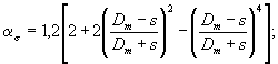
σψp is
calculated by the formula in item 2.3.2.1.
Parameter
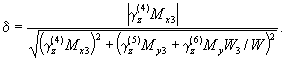
The meaning of
other values is explained in item 2.9.3.1.
2.9.3.3. Components of
the reduced stresses (amplitude values) are determined by the formulas (from
pressure, mechanical and temperature effects)
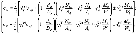
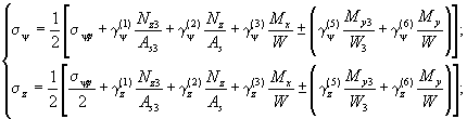
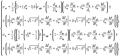
At Dm/dm
< 1.3, the following stresses are additionally calculated:
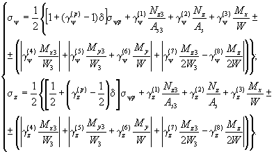
The values in
the formulas have the same meaning as in item 2.9.3.2, the torsion
stresses τ are reduced by 2 times, σr = 0.
2.9.3.4.
Coefficients of local stresses γψ(i), γz(i),
γψz(i) (i =p, 1, 4, 5, 7) are
determined by the formula
γ(i)(ss/dm,
s/Dm, Dm/dm) = K(i)(ssDm/sdm)γi(ss/dm,
Dm/dm),
coefficients K(i),
γiψ, γiz, γiψz,
γ(j)ψ, γ(j)z
and γ(j)ψz (j = 2, 3, 6, 8) are determined
by the nomograms shown in Fig. P5.8 - P5.14. For equal and
similar tees (ss/dm ≈ s/Dm)
it shall be assumed that K(i) = 1. Coefficients γ(ss/dm,
Dm/dm) for "intermediate" values
of ss/dm (ss1/dm1
< ss/dm < ss2
/dm2) are determined by linear interpolation by
coefficients γ1 (ss1/dm1,
Dm/dm) and γ2 (ss2/dm2,
Dm/dm):
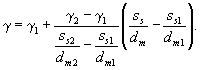
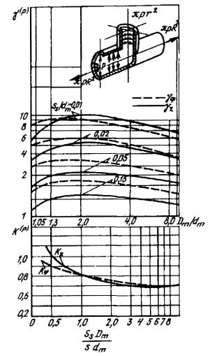
Fig. P5.8.
Nomograms to determine the coefficients γ(p) and K(p)
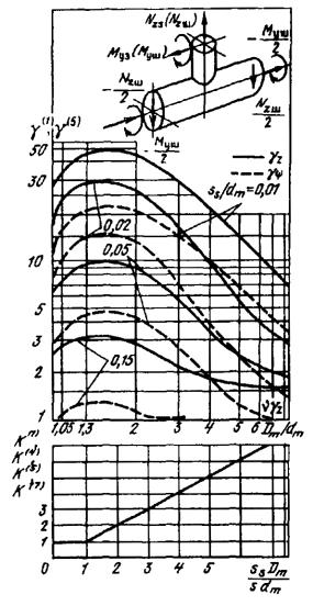
Fig. P5.9.
Nomograms to determine the coefficients γ(1), γ(5), K(1),
K(4), K(5) and K(7)
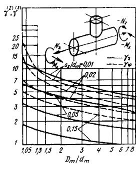
Fig. P5.10.
Nomograms to determine the coefficients γ(2) and γ(3)
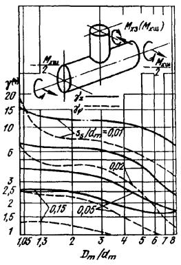
Fig. P5.11.
Nomograms to determine the coefficient γ(4)
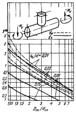
Fig. P5.12.
Nomograms to determine the coefficient γ(6)
The following
conditions shall be met for all tees
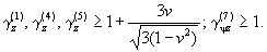
For
essentially unequal tees (Dm/dm ≥ 8), it is
allowed to assume that γψб) = γz(6)
= 0 at any ratios of s/Dm and ss/dm;
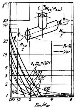
Fig. P5.13.
Nomograms to determine the coefficient γ(7)
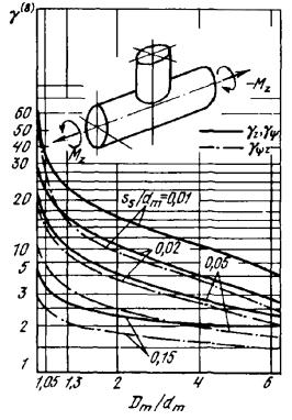
Fig. P5.14.
Nomograms to determine the coefficient γ(8)
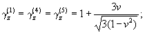
γψ(1)
= γψ(4) = γψ(5) = vγz(1);
γψ(2)
= γψ(3) = γz(2) = γz(3)
= 3;
γψ(7)
= γz(7) = 0, γψz(7) = 1;
γψ(8)
= -γz(8) = 2, γψz(7)
= 0
at s/Dm
> 2ss/dm (v is a Poisson ratio).
2.10. SPECIAL CALCULATIONS OF PIPELINES
2.10.1. For the
abnormal operation mode, the requirements of items 2.3.1 and 2.3.4
shall be met, provided that the maximum pressure for the considered mode is
entered into the calculation, and the permissible stress is taken according to
item 5.4 hereof.
2.10.2. When
considering the load cases, including the action of seismic loads, the
calculation of stresses is carried out according to the formulas in items 2.3.1
and 2.3.4. Permissible stresses are assumed in accordance with item 5.11
hereof.
2.10.3. A pipeline
strength verification is required for stress category (σ)2 for
hydrotest conditions. The calculation is performed on the combined effect of
pressure and mass load. The strength condition is assumed according to item 5.4
hereof.
3. DETACHABLE CONNECTIONS
OF VESSELS
3.1. CONVENTION SYMBOLS
Fob is a force required for
gasket compression, N (kgf)
Fpr.p is a gasket
force ensuring tightness in service conditions, N (kgf)
Fp is a hydrostatic force
in operating modes, N (kgf)
Fpr is a hydrostatic force
during hydrotest, N (kgf)
p is a design
pressure, Pa (kgf/mm2)
ph is a
hydrotest pressure, Pa (kgf/mm2)
F0w is a force of initial
tightening of pins, N (kgf)
Fw is a pin force, N (kgf)
Fpr is an axial force on
the gasket, N (kgf)
Qpr is a radial force on a
wedge piece, N (kgf)
FT is a pin force caused by temperature differences,
N (kgf)
χ is a load coefficient
λpr is
a gasket compliance coefficient, mm/N (mm/kgf)
λr is
a barrel jacket compliance coefficient, mm/N (mm/kgf)
λw is
a pin compliance coefficient, mm/N (mm/kgf)
λb is
a bush (washer) compliance coefficient, mm/N (mm/kgf)
Er is a modulus of
longitudinal elasticity of the material of a jacket, Pa (kgf/mm2)
Ew is a modulus of
longitudinal elasticity of the material of a pin, Pa (kgf/mm)
Epr is a modulus of
longitudinal elasticity of the material of a gasket, Pa (kgf/mm2)
Fpr.h is a gasket
force ensuring tightness during hydrotest, N (kgf)
λf is
a pressure flange compliance coefficient, mm/N (mm/kgf)
Ef is a modulus of
longitudinal elasticity of the material of a pressure flange, Pa (kgf/mm2)
Eb is a modulus of
longitudinal elasticity of the material of a bush (washer), Pa (kgf/mm2)
hpr is a design
height of a gasket, mm
hb is a height
of a bush (washer), mm
Ab is a cross-sectional
area of a bush (washer), mm2
Δl1 is
a total vertical temperature expansion of the body and pin on the segment
between the support clamp of the body and the bottom end of the nut, mm
Δl2 is
a total vertical temperature expansion of the lid, gasket, pressure flange,
bush and clamp (for the case the clamp is on the anti-corrosion jacket) on the
segment between the support clamp of the body and the bottom end of the nut, mm
Dpr is a mean diameter of
gasket, mm
z is a number
of pins;
b1 is a design
width of gasket, mm
b0 is a
conditional width of gasket, mm
b is an
effective width of gasket, mm
h1 is a height
of a wedge piece, mm
b2 is a width
of a cone of a wedge piece, mm
b'1 is a total
width of grooves on a gasket or contacting surface along the width b1,
mm
b'2 is a total
width of grooves on a cone of a wedge piece, mm
h'1 is a total
width of grooves on a cylindrical surface of a wedge piece, mm
α is an angle of a cone
of a wedge piece, deg
m is a gasket
coefficient
q0 is a
specific pressure on the gasket during compression, Pa (kgf/mm2)
l is a free
length of a pin – pin rod length between the bottom end of the nut and the
upper end of the body, mm
dw is a pin rod
diameter, mm
d0 is an outer
diameter of a pin thread, mm
d1 is an inner
diameter of a pin thread, mm
Aw is a pin rod
cross-sectional area, mm2
W is a pin rod cross-section resistance moment
when bending, mm3
Wk is a pin rod
cross-section resistance moment when torsion, mm3
J is a pin rod cross-section inertia moment when
bending, mm
Mk is a torque affecting a
pin, N · mm (kgf · mm)
M1, M2 is a pin bending
moments, N · mm (kgf · mm)
w1 is a radial
displacement of the flange end of a body, mm
w2 is a radial
displacement of the lower end of a nut, mm
θ1 is an
angular displacement of the flange end of a body, rad
θ2 is an
angular displacement of the lower end of a nut, rad
σmw is
a tension stress in pins, Pa (kgf/mm2)
σbw is
a bending stress in pins, Pa (kgf/mm2)
τsw is a torsion
stress in pins, Pa (kgf/mm2)
h' is a height
of the operating part of a thread (threaded connection), mm
Jf is a pressure flange
cross-section inertia moment relative to the horizontal axis passing through
the center of gravity, mm4
R is a radius of the center of mass of a pressure
flange cross-section, mm
Fig. P5.15.
Standard designs of flange connections:
a – with a
flat gasket; b – with a wedge piece; c – with a flexible sealing
component:
1 – body flange; 2
– pin; 3 – bush (washer); 4 – gasket; 5 – lid; 6 –
body flange; 7 – flexible sealing component
3.2. GENERAL
3.2.1. The
procedure applies to detachable connections of vessels and devices operating
under inner pressure at temperatures below Tt.
Standard
designs of connection are shown in Fig. P5.15.
3.3. CALCULATION OF DETACHABLE CONNECTION
Calculate the
efforts of the initial tightening of pins, the efforts in pins and on gasket
under operating conditions, as well as the stresses in pins.
3.4. CALCULATION OF LOAD COEFFICIENT
3.4.1. The load
coefficient takes into account the effect of internal pressure on the forces in
pins and on gasket of a pre-tightened connection.
Coefficient:
of load shall be determined by the formula
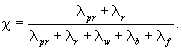
3.4.2. The
coefficient of compliance of gasket λpr for the case when the
gasket is installed between the lid and supporting clamp of the body is
calculated by the formula

where Apr
= pDprb is a cross-sectional area of the gasket.

Fig. P5.16.
Body flange with anti-corrosion jacket
|
рубашка
корпуса
|
body jacket
|
For a wedge
seal and gasketless connection with a flexible sealing component, it is assumed
that λpr = 0.
3.4.3. Coefficient
of compliance of body clamp λr with anti-corrosion jacket
(Fig. P5.16) is calculated by the formula
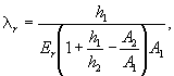
where h1,
h2 is a component jacket height; A1, A2
is a cross-sectional area of a jacket component. If the clamp is on the body
having no jacket, then it is assumed that λr = 0.
3.4.4. Coefficient
of compliance of pin λw, taking into account the compliance
of the pin rod and threaded connection pin-body and pin-nut, is calculated by
the formula
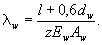
3.4.5. The
coefficient of compliance of bush (washer) is calculated by the formula

3.4.6. The
coefficient of compliance of pressure flange

where a is a size
shown in Fig. P5.16.
3.5. CALCULATION OF FORCES IN PINS CAUSED BY
TEMPERATURE DIFFERENCES
Forces in pins
caused by temperature differences in the parts of connection or by difference
in the linear expansion coefficients of the materials of the parts of
connection are determined by the formula
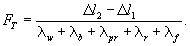
An example of
dividing a connection into sections for calculating temperature expansions is
shown in Fig. P5.16.
For this
example Δl1 = α1l1T1
+ α2l2T2, Δl2
= α3l3T3 + α4l4T4
+ α5l5T5 + α6l6T6
+ α7l7T7, where α1, li,
Ti – coefficient of linear expansion of the material, length
of sections, and mean temperature in the section.
Coefficients
of compliance λw, λb, λpr,
λr and λf are calculated in accordance with
items 3.4.2 - 3.4.6.
3.6. CALCULATION OF FORCES OF INITIAL TIGHTENING OF
PINS
3.6.1. The initial
tightness of connection is carried out to eliminate the leakiness of the gasket
against the contacting surfaces and to create conditions ensuring resistance of
the joint and tightness of the connection during hydrotests or action of the
operating pressure and temperature differences.
3.6.2. The force
required to compress the gasket,
F0b = pDprbq0.
3.6.3. Force on
the gasket (except self-sealing wedge one), ensuring tightness at operating
pressure and hydrotest,
Fpr.p = pDprbmp;
Fpr.h = pDprbmhh.
For
self-sealing wedge piece
Fpr.p = Fpr.h
= 0.
3.6.4. The values
of b, m, q0 are selected from Table P5.6.
Table P5.6. Values
of b, m and q0 for different types of gaskets
|
Type
of gasket
|
Design of
gasket
|
Material
|
Effective
width b, mm
|
Liquid media
|
Air,
steam, steam and water mixture
|
Highly
penetrating gases (hydrogen, helium, etc.)
|
|
m
|
q0, MPa
|
m
|
q0, MPa
|
m
|
q0, MPa
|
|
Soft
|
Flat

|
Solid rubber
|
b0
|
1.2
|
5
|
2.2
|
9
|
3.0
|
13
|
|
Fluoropolymer
|
1.4
|
10
|
2.5
|
18
|
3.1
|
26
|
|
Paronite
|
b0 at b0
≤ 10
 at b0
> 10 at b0
> 10
|
1.6
|

|
2.9
|

|
4
|

|
|
Combined
|
Spiral

|
Pearlite steel
|
|
1.5
|
27
|
2.5
|
50
|
4
|
70
|
|
Corrugated ribbon
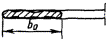
|
Aluminum, its alloys
|
|
1.75
|
20
|
3.0
|
30
|
4.25
|
42
|
|
Copper, its alloys
|
b0
|
1.9
|
20
|
3.25
|
35
|
4.5
|
50
|
|
Pearlite steel
|
|
2.0
|
22
|
3.5
|
40
|
5
|
55
|
|
With an outer metal
shell
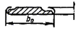
|
Aluminum, its alloys
|
|
1.9
|
27
|
3.25
|
50
|
4.5
|
70
|
|
Copper, its alloys
|
|
2.0
|
32
|
3.5
|
60
|
5
|
80
|
|
Pearlite steel
|
|
2.25
|
38
|
3.75
|
70
|
5.5
|
100
|
|
Metal
|
Shaped (circle,
oval, octangle)
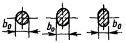
|
Copper, its alloys;
nickel, its alloys
|
0.6b0
|
2.5
|
2.4Rр0.2
|
4.5
|
3Rp0.2
|
6
|
4Rр0.2
|
|
Pearlite steel
|
3.0
|
5.0
|
7
|
|
Austenitic steel
|
3.5
|
6.0
|
8
|
|
Flat

Wedge
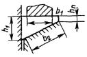
|
Aluminum, its alloys
|
b0 at b0
≤ 10
|
2.0
|

|
3.5
|

|
5
|

|
|
Copper, its alloys;
nickel, its alloys
|
at b0
> 10
|
2.5
|
4.5
|
6
|
|
Pearlite steel
|
|
3.0
|
5.0
|
7
|
|
Austenitic steel
|
|
3.5
|
6.0
|
8
|
|
|
Toothed, with number
of teeth of zn

|
Copper, its alloys;
nickel, its alloys
|
|
1.8
|
2.4Rр0.2
|
3.3
|
3Rp0.2
|
4.6
|
4Rр0.2
|
|
Pearlite steel
|
2.25
|
3.75
|
5.5
|
|
Austenitic steel
|
2.5
|
4.25
|
6
|
|
Note. For wedge piece b0
= max{b2 sinα; h1 tgα} in the presence of
grooves on the gasket or on contacting surfaces instead of values of h1,
b1, b2, the following is used h1 –
h'1, b1 – b'1, b2
– b'2, when determining q0, it
is assumed that δ = b0.
|
3.6.5. Hydrostatic
forces from operating pressure and hydrotest pressure
Fp = 0.785D2prp;
Fph = 0.785D2prph.
3.6.6. Force of
initial tightening of pins shall be selected from the conditions
F0w ≥ Fob,
F0w ≥ Fpr.h
+ (1 – χ)Fph.
3.6.7. To maintain
tightness, the following condition shall be maintained
F0w ≥ Fpr.p
+ (1 – χ)Fp – FT.
If this
condition is not satisfied, then you shall make structural changes to the
connection or change the temperature operation modes of the connection.
If necessary,
it is allowed to increase initial tightening force in accordance with the above
condition.
3.7. CALCULATION
OF GASKET FORCES
3.7.1. Gasket
force when tightening
Fpr = F0w.
3.7.2. Gasket
force during hydrotest:
Fpr = F0w
+ χFph – for wedge piece;
Fpr = F0w
- (1 - χ)Fph – for other types of gaskets.
3.7.3. Gasket force
in service conditions:
Fpr = F0w
+ χFp +FT – for wedge piece;
Fpr = F0w
- (1 - χ)Fp + FT – for other types of
gaskets.
3.7.4. For the
wedge piece, in addition to axial forces, radial forces are determined:
radial force during
initial tightening
Qpr = F0w/tg
α;;
radial force during
hydrotest
Qpr = [F0w
+ χFph]/tg α;
radial force in service
conditions
Qpr = (F0w
+ χFp + FT)/tg α.
3.7.5. Flat
gaskets and wedge pieces are checked for the specific pressure on the contact
surfaces during tightening, hydrotest and operating modes.
Specific
pressure on flat gasket

Specific
pressure on wedge piece
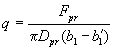 – for a flat
contact surface;
– for a flat
contact surface;
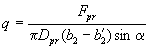 – for a cone
contact surface;
– for a cone
contact surface;
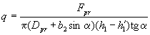 – for a
cylindrical contact surface.
– for a
cylindrical contact surface.
The following
two conditions shall be met:
1) q ≥ qminK,
where qmin is a minimum permissible specific pressure on the
gasket from the condition of tightness of the detachable connection; K
is a coefficient depending on the penetrating ability of the sealed medium;
2) q ≤ qmax,
where qmax is a maximum permissible specific pressure on the
gasket from the condition of its working capacity (Table P5.7).
The following
values of coefficient K are recommended:
K = 1 – for liquid medium;
K = 1.8 – for extremely penetrating air;
(hydrogen, helium, etc.).
Table P5.7. Values
of qmin and qmax
|
Gasket
material
|
qmin, MPa
|
qmax, MPa
|
|
Solid rubber
|
3.5
|
20.0
|
|
Fluoropolymer
|
4.0
|
40.0
|
|
Paronite
|
10.0
|
110.0
|
|
Aluminum and its
alloys
|
50.0
|
140.0
|
|
Copper and its alloys
|
70.0
|
200.0
|
|
Pearlite steel
|
80.0
|
350.0
|
|
Austenitic steel
|
100.0
|
600.0
|
For a wedge
piece, the specific pressure for a flat contact surface is checked only by
condition 2.
If the
verification on the specific pressure on the contact surfaces gives negative
results, you shall perform structural changes to the connection or change the
temperature conditions of the connection. If necessary, it is allowed to
increase the force of initial tightness F0w.
After
performing at least one of these measures, the calculation shall be repeated.
3.8. CALCULATION OF FORCES IN PINS
3.8.1. Pin force
when tightening
Fw = F0w.
3.8.2. Pin force
during hydrotest
Fw = F0w
+ χFph.
3.8.3. Pin force
in service conditions
Fw = F0w
+ χFp + FT.
3.9. CALCULATION OF STRESSES IN PINS
3.9.1. Calculation
of pin rod
3.9.1.1. Torque
affecting the pin when tightening the nuts with a wrench,
Mk = zFowd0/z,
where z is selected
according to Table P5.8.
Tong torque
when tightening the nuts
Mtg = z1F0wd0/z,
where z1 is
selected according to Table P5.8.
Table P5.8. Values
of coefficients z and z1
|
Grease
|
z
|
z1
|
|
Yes
|
0.13
|
0.26
|
|
None
|
0.18
|
0.37
|
When
tightening pins with pre-heating or pre-stretching Mk = 0.
3.9.1.2. Bending
moments in pin are calculated by the formulas
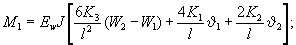
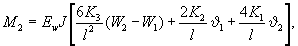
where J = 0.049d4pin;
K1 = K2
= K3 = 1 for 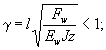

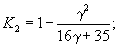
 for 1 ≤
γ ≤ 6;
for 1 ≤
γ ≤ 6;


 for γ
> 6.
for γ
> 6.
W1, W2,  ,
,  are
determined from the condition of compatibility of the connection deformation.
are
determined from the condition of compatibility of the connection deformation.
Positive
directions of displacements and angles of rotation adopted in the formulas are
shown in Fig. P5.17.
3.9.1.3.
Tension stress

where Aw
= 0.785d12.
3.9.1.4. Torsion
stress

where Wk
= 0.196d13.
3.9.1.5. Bending
stress

where W = 0.1d13.
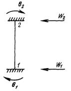
Fig. P5.17.
Positive directions of displacements and joints of rotation of pin
3.9.2. Calculation
of pin thread
3.9.2.1. Thread cut
tension
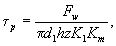
where K1
is a thread completeness coefficient; K1 = 0.87 – for metric
thread (nut); K1 = 0.75 – for metric thread (bolts, pins); K1
= 0.4 – for rectangular thread; K1 = 0.65 – for trapezoidal
thread; Km is a coefficient taking into account change in the
deformation of coils along the height of the nut (Table P5.9).
Table P5.9. Value
of coefficient Km
|
Rmb/Rmn
|
Thread
pitch
|
Km
|
|
Over 1.3
|
Large and first small
Second and smaller
|
0.7 - 0.75
0.65 - 0.7
|
|
Less than 1.3
|
For all pitches
|
0.55 - 0.6
|
Note. Rmb,
Rmn are the strength limits of bolt and nut.
APPENDIX 6
CHARACTERISTICS OF LONG-TERM STRENGTH,
DUCTILITY AND CREEP OF STRUCTURAL MATERIALS
1. BASIC CONCEPTS AND
SYMBOLS
σ is a stress, MPa
(kgf/mm2)
RTmt is a
specific limit of long-term durability over time t at temperature T,
MPa (kgf/mm2)
 is a conditional
creep limit at temperature T for time TAz
of achievement of a given deformation Az, MPa (kgf/mm2)
is a conditional
creep limit at temperature T for time TAz
of achievement of a given deformation Az, MPa (kgf/mm2)
T is a temperature, K (°C)
tT is a current
test time, h
tc is time to
fracture, h
tT, tT1
is a current test time at temperatures T, T1, h
t is time to
reach the specified residual elongation Az, h
tTz is a given
operation life at temperature Tj, h
e –
deformation, %
 is a creep rate,
%/h
is a creep rate,
%/h
A is a relative tension elongation, %
AtT is a
conditional limit of residual elongation at rupture at temperature Tj,
%
Az is a specified residual elongation, %
Z is a relative contraction of the sample
cross-sectional area at rupture, %
ZtT is a
conditional limit of long-term static contraction at temperature T over
time t, %
|


|

|
are heat resistance
characteristics at temperature T, for a given level of probability of
destruction Р and operation life tz, MPa (kgf/mm2),
%
|
γl-t.s is an extrapolation
coefficient of long-term strength
γc is an
extrapolation coefficient of creep
|
 
|
|
is a standard
deviations of heat resistance characteristics
|
nT is a number
of experiments at temperature T
P is a probability of destruction
M is a number of batches
2. GENERAL
2.1. This
Appendix to the rules of equipment and pipelines strength calculation of
nuclear power plants contains the methods for obtaining the heat resistance
characteristics of structural materials. A temperature range of 573–923 K (300–
650 °C) is considered, at which creep and long-term strength appear in the
metal.
2.2. To
determine the heat resistance characteristics with probability of P =
0.5 and P = 0.01 (conditional strength limit, conditional creep limit,
conditional limits of relative lengthening and contraction) it is allowed to
use parametric methods in accordance with OST 108.901.102-78 (Section 5).
2.3. The number
of samples when testing one batch is distributed evenly over the stresses
corresponding to the durability from 102 to 104 h and
more, so that for every order in time the number of stress levels was at least
two.
Minimum number
of tested samples shall be 12.
2.4. It each
mode, at least two samples are tested. If the times to failure of samples
tested in the same mode differ by more than 2 times, then additional tests are
carried out on two samples.
When
processing the test results, all the results obtained in the main and
additional tests are considered.
2.5. Tests to
obtain the conditional creep limit are carried out with the measurement of
deformation according to GOST 3248-81.
2.6. Samples are
tested at temperature T1 for which the heat resistance
characteristics are determined, and at a higher temperature
T2 = T1
+ 50 K.
2.7. The
proposed method for determining the heat resistance characteristics of
materials allows extrapolation by the parameter t within the same order,
but up to stresses not lower than the minimum stresses obtained during
long-term strength tests at temperature T2.
2.8. In order to
obtain guaranteed heat resistance characteristics of steel or alloy, test
results obtained for different batches representing a steel or alloy grade of a
given strength category are considered legitimate. The number of tested batches
of metal of various fusions shall be at least six.
The number of
tested includes batches and metal of products after the final process
operations with the content of carbon and alloying components and the values of
short-term strength and ductility within the limits specified in the technical
specifications (TU).
2.9. In the
absence of direct tests to determine the heat resistance characteristics of
steel or alloy of strength category given below in Table P1.4 hereof,
their limits of long-term strength are determined by the values of the limits
of long-term strength of grade of steel or alloy of strength category specified
in Table P1.4 hereof, and their temporary resistance and yield limits.
The desired value is assumed as the minimum of two (quantities) defined by the
formulas
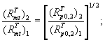
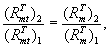
where index 1 is the
strength category given in Table P1.4 hereof (strength category 1);
index 2 is a strength category for which heat resistance characteristics are
calculated (strength category 2); (RTmt)1,
(RTmt)2, (RTp0.2)1,
(RTp0.2)2, (RTm)1,
(RTm)2 are, respectively, the limits of
long-term strength, yield and temporary resistance of metal of strength
categories 1 and 2. Values of the required characteristics are selected
according to Tables P1.1 and P1.4 hereof.
In the same
way, the value of long-term ductility (relative elongation AtT
and contraction ZtT) of a metal of strength
category 2 is allowed to be determined from known values of the limits of
relative elongation (contraction) of a metal under strength category 1,
temporary resistance and yield limit of metal of strength categories 1 and 2.
The desired value is assumed as the minimum of two characteristics defined by
the formulas:
for ZtT
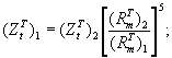
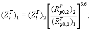
for AtT
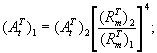
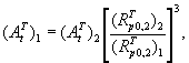
where (ZtT)1,
(ZtT)2, (AtT)1,
(AtT)2 are, respectively, the limits of
long-term relative contraction and elongation of metal of strength categories 1
and 2.
Values of (AtT)1
and (ZtT)1 are taken according to Table
P6.3. For metal of strength category given above in Table P1.4
hereof, the values of RTmt, ZtT
and AtT are selected in accordance with those in Table
P1.1 hereof and Table P6.3.
2.10. This
Appendix provides:
tables of mean values of
limits of long-term strength over a period of time from 10 to 2 · 105
h (Table P6.1, P6.2);
curves of long-term
strength (at the minimum values of Fig. P6.1 - P6.17);
tables of mean values of
limits of long-term ductility on the basis of 2 · 105 h (Table P6.3,
P6.4);
isochronous deformation
(creep) curves plotted at a given temperature by the time parameter in the
coordinates σ - e by mean values (Fig. P6.18 - P6.29);
extrapolation methods
for long times of characteristics of long-term strength, ductility and creep.
Heat
resistance characteristics are used:
Table P6.1. Mean
values of conditional limits of long-term strength RTmt,
MPa (kgf/mm2)
|
Steel,
alloy grade
|
R20p0.2, MPa
(kgf/mm2)
|
Rm20, MPa
(kgf/mm2)
|
Temperature,
K (°C)
|
Time, h
|
|
10
|
30
|
102
|
3 · 102
|
103
|
3 · 103
|
104
|
3 · 104
|
105
|
2 · 105
|
|
15KhM
|
≥ 235
|
≥ 441
|
773
|
412
|
402
|
372
|
348
|
314
|
260
|
217
|
183
|
142
|
120
|
|
|
(24)
|
(45)
|
(500)
|
(42)
|
(41)
|
(38)
|
(35.5)
|
(32)
|
(26.5)
|
(22.1)
|
(18.7)
|
(14.5)
|
(12.2)
|
|
12MKh
|
≥ 225
|
≥ 411
|
773
|
368
|
368
|
353
|
328
|
299
|
274
|
207
|
174
|
135
|
114
|
|
|
(23)
|
(42)
|
(500)
|
(37)
|
(37)
|
(36)
|
(33.5)
|
(30.5)
|
(28)
|
(21.1)
|
(17.8)
|
(13.8)
|
(11.6)
|
|
10Kh2M
|
≥ 245
|
≥ 392
|
723
|
372
|
353
|
333
|
314
|
294
|
274
|
255
|
225
|
196
|
186
|
|
(48TN-1)
|
(25)
|
(40)
|
(450)
|
(38)
|
(36)
|
(34)
|
(32)
|
(30)
|
(28)
|
(26)
|
(23)
|
(20)
|
(19)
|
|
|
|
|
773
|
353
|
313
|
284
|
255
|
216
|
186
|
157
|
137
|
118
|
108
|
|
|
|
|
(500)
|
(36)
|
(32)
|
(29)
|
(26)
|
(22)
|
(19)
|
(16)
|
(14)
|
(12)
|
(11)
|
|
|
|
|
783
|
319
|
289
|
261
|
234
|
201
|
172
|
145
|
126
|
108
|
99
|
|
|
|
|
(510)
|
(32.5)
|
(29.5)
|
(26.6)
|
(23.9)
|
(20.5)
|
(17.5)
|
(14.8)
|
(12.9)
|
(11)
|
(10.1)
|
|
12Kh2M
|
≥ 343
|
≥ 539
|
773
|
451
|
431
|
412
|
353
|
294
|
265
|
216
|
177
|
147
|
132
|
|
|
(35)
|
(55)
|
(500)
|
(46)
|
(44)
|
(42)
|
(36)
|
(30)
|
(27)
|
(22)
|
(18)
|
(15)
|
(13.5)
|
|
|
≥ 255
|
≥ 451
|
773
|
392
|
372
|
343
|
294
|
255
|
216
|
177
|
147
|
118
|
105
|
|
|
(25)
|
(46)
|
(500)
|
(40)
|
(38)
|
(35)
|
(30)
|
(26)
|
(22)
|
(18)
|
(15)
|
(12)
|
(10.7)
|
|
10Kh2M1FB
|
≥ 196
|
≥ 343
|
673
|
333
|
319
|
304
|
297
|
284
|
268
|
235
|
212
|
186
|
167
|
|
(48TN-2)
|
(20)
|
(35)
|
(400)
|
(34)
|
(33)
|
(31)
|
(30)
|
(29)
|
(27)
|
(24)
|
(22)
|
(19)
|
(17)
|
|
|
|
|
723
|
333
|
314
|
299
|
294
|
269
|
250
|
225
|
201
|
176
|
167
|
|
|
|
|
(450)
|
(34)
|
(32)
|
(30.5)
|
(30)
|
(27.5)
|
(25.5)
|
(23)
|
(20.5)
|
(18)
|
(17)
|
|
|
|
|
773
|
250
|
230
|
201
|
181
|
162
|
147
|
132
|
122
|
108
|
98
|
|
|
|
|
(500)
|
(25.5)
|
(23.5)
|
(20.5)
|
(18.5)
|
(16.5)
|
(15)
|
(13.5)
|
(12.5)
|
(11)
|
(10)
|
|
|
|
|
823
|
216
|
196
|
167
|
147
|
127
|
113
|
98
|
83
|
78
|
70
|
|
|
|
|
(550)
|
(22)
|
(20)
|
(17)
|
(15)
|
(13)
|
(11.5)
|
(10)
|
(8.5)
|
(8)
|
(7.2)
|
|
12Kh1MF
|
≥ 274
|
≥ 441
|
723
|
353
|
343
|
323
|
303
|
289
|
268
|
245
|
227
|
196
|
186
|
|
|
(28)
|
(45)
|
(450)
|
(36)
|
(35)
|
(33)
|
(31)
|
(29.5)
|
(27.5)
|
(25)
|
(23.5)
|
(20)
|
(19)
|
|
|
|
|
773
|
353
|
343
|
323
|
304
|
279
|
260
|
216
|
186
|
147
|
137
|
|
|
|
|
(500)
|
(36)
|
(35)
|
(33)
|
(31)
|
(28.5)
|
(26.5)
|
(22)
|
(19)
|
(15)
|
(14)
|
|
12Kh18N10T
|
≥ 216
|
≥ 529
|
673
|
372
|
372
|
372
|
372
|
372
|
372
|
372
|
372
|
372
|
372
|
|
12Kh18N12T
|
(22)
|
(54)
|
(400)
|
(38)
|
(38)
|
(38)
|
(38)
|
(38)
|
(38)
|
(38)
|
(38)
|
(38)
|
(38)
|
|
|
|
|
723
|
372
|
372
|
372
|
372
|
372
|
372
|
372
|
372
|
333
|
314
|
|
|
|
|
(450)
|
(38)
|
(38)
|
(38)
|
(38)
|
(38)
|
(38)
|
(38)
|
(38)
|
(34)
|
(32)
|
|
|
|
|
773
|
372
|
352
|
333
|
323
|
314
|
284
|
255
|
225
|
196
|
186
|
|
|
|
|
(500)
|
(38)
|
(36)
|
(34)
|
(33)
|
(32)
|
(29)
|
(26)
|
(23)
|
(20)
|
(19)
|
|
|
|
|
823
|
353
|
333
|
314
|
294
|
265
|
235
|
201
|
171
|
149
|
137
|
|
|
|
|
(550)
|
(36)
|
(34)
|
(32)
|
(30)
|
(27)
|
(24)
|
(20.5)
|
(17.5)
|
(15.2)
|
(14)
|
|
|
|
|
873
|
314
|
284
|
255
|
240
|
216
|
186
|
157
|
127
|
108
|
97
|
|
|
|
|
(600)
|
(32)
|
(29)
|
(26)
|
(24.5)
|
(22)
|
(19)
|
(16)
|
(13)
|
(11)
|
(9.9)
|
|
08Kh16N11M3
|
≥ 196
|
≥ 510
|
673
|
392
|
392
|
392
|
392
|
392
|
392
|
392
|
392
|
392
|
392
|
|
(20)
|
(52)
|
(400)
|
(40)
|
(40)
|
(40)
|
(40)
|
(40)
|
(40)
|
(40)
|
(40)
|
(40)
|
(40)
|
|
|
|
|
723
|
372
|
372
|
372
|
372
|
372
|
353
|
343
|
314
|
294
|
284
|
|
|
|
|
(450)
|
(38)
|
(38)
|
(38)
|
(38)
|
(38)
|
(36)
|
(35)
|
(32)
|
(30)
|
(29)
|
|
|
|
|
773
|
372
|
372
|
372
|
343
|
323
|
304
|
284
|
245
|
220
|
196
|
|
|
|
|
(500)
|
(38)
|
(38)
|
(38)
|
(35)
|
(33)
|
(31)
|
(29)
|
(25)
|
(22.5)
|
(20)
|
|
|
|
|
823
|
332
|
304
|
274
|
260
|
245
|
230
|
216
|
191
|
167
|
157
|
|
|
|
|
(550)
|
(34)
|
(31)
|
(28)
|
(26.5)
|
(25)
|
(23.5)
|
(22)
|
(19.5)
|
(17)
|
(16)
|
|
|
|
|
873
|
265
|
240
|
216
|
196
|
167
|
157
|
137
|
110
|
108
|
96
|
|
|
|
|
(600)
|
(27)
|
(24.5)
|
(22)
|
(20)
|
(17)
|
(16)
|
(14)
|
(12)
|
(11)
|
(10)
|
|
15Kh1M1F
|
≥ 314
|
≥ 490
|
773
|
363
|
343
|
333
|
314
|
288
|
270
|
240
|
225
|
196
|
184
|
|
|
(32)
|
(50)
|
(500)
|
(37)
|
(35)
|
(34)
|
(32)
|
(29.4)
|
(27.5)
|
(24.5)
|
(23)
|
(20.1)
|
(18.8)
|
|
12Kh18N9
|
196
|
>490
|
673
|
373
|
373
|
373
|
373
|
373
|
373
|
373
|
373
|
373
|
373
|
|
|
(20)
|
(50)
|
(400)
|
(38)
|
(38)
|
(38)
|
(38)
|
(38)
|
(38)
|
(38)
|
(38)
|
(38)
|
(38)
|
|
|
|
|
723
|
373
|
373
|
373
|
373
|
373
|
373
|
373
|
323
|
303
|
274
|
|
|
|
|
(450)
|
(38)
|
(38)
|
(38)
|
(38)
|
(38)
|
(38)
|
(38)
|
(33)
|
(31)
|
(28)
|
|
|
|
|
773
|
373
|
353
|
343
|
323
|
294
|
265
|
245
|
216
|
196
|
186
|
|
|
|
|
(500)
|
(38)
|
(36)
|
(35)
|
(33)
|
(30)
|
(27)
|
(25)
|
(22)
|
(20)
|
(19)
|
|
|
|
|
823
|
333
|
323
|
298
|
284
|
245
|
206
|
176
|
157
|
137
|
127
|
|
|
|
|
(550)
|
(34)
|
(33)
|
(30.5)
|
(29)
|
(25)
|
(21)
|
(18)
|
(16)
|
(14)
|
(13)
|
|
|
|
|
873
|
274
|
265
|
240
|
201
|
172
|
157
|
123
|
108
|
88
|
78
|
|
|
|
|
(600)
|
(28)
|
(27)
|
(24.5)
|
(20.5)
|
(17.5)
|
(16)
|
(12.5)
|
(11)
|
(9)
|
(8)
|
|
10Kh17N13M2T
|
≥ 196
|
≥ 510
|
773
|
304
|
284
|
265
|
250
|
235
|
216
|
201
|
176
|
157
|
147
|
|
(20)
|
(52)
|
(500)
|
(31)
|
(29)
|
(27)
|
(25.5)
|
(24)
|
(22)
|
(20.5)
|
(18)
|
(16)
|
(15)
|
|
|
|
|
823
|
255
|
235
|
216
|
196
|
176
|
162
|
147
|
129
|
118
|
108
|
|
|
|
|
(550)
|
(26)
|
(24)
|
(22)
|
(20)
|
(18)
|
(16.5)
|
(15)
|
(13.2)
|
(12)
|
(11)
|
|
|
|
|
873
|
221
|
203
|
186
|
167
|
152
|
132
|
113
|
98
|
83
|
77
|
|
|
|
|
(600)
|
(22.5)
|
(20.7)
|
(19)
|
(17)
|
(15.5)
|
(13.5)
|
(11.5)
|
(10)
|
(8.5)
|
(7.9)
|
|
KhN35VT
|
≥ 392
|
≥ 736
|
673
|
645
|
645
|
645
|
645
|
645
|
645
|
645
|
645
|
627
|
588
|
|
|
(40)
|
(75)
|
(400)
|
(66)
|
(66)
|
(66)
|
(66)
|
(66)
|
(66)
|
(66)
|
(66)
|
(64)
|
(60)
|
|
|
|
|
723
|
637
|
637
|
637
|
637
|
637
|
637
|
625
|
568
|
549
|
530
|
|
|
|
|
(450)
|
(65)
|
(65)
|
(65)
|
(65)
|
(65)
|
(65)
|
(62.5)
|
(58)
|
(56)
|
(54)
|
|
|
|
|
773
|
637
|
588
|
549
|
529
|
500
|
480
|
451
|
412
|
343
|
323
|
|
|
|
|
(500)
|
(65)
|
(60)
|
(56)
|
(54)
|
(51)
|
(49)
|
(46)
|
(42)
|
(35)
|
(33)
|
|
|
|
|
823
|
539
|
529
|
490
|
470
|
441
|
417
|
372
|
333
|
304
|
284
|
|
|
|
|
(550)
|
(55)
|
(54)
|
(50)
|
(48)
|
(45)
|
(42)
|
(38)
|
(34)
|
(31)
|
(29)
|
|
|
|
|
873
|
431
|
412
|
392
|
363
|
343
|
314
|
294
|
250
|
216
|
196
|
|
|
|
|
(600)
|
(44)
|
(42)
|
(40)
|
(37)
|
(35)
|
(32)
|
(30)
|
(25.5)
|
(22)
|
(20)
|
|
1Kh16N36MBTYUR
|
≥ 392
|
≥ 785
|
773
|
884
|
850
|
824
|
808
|
794
|
768
|
612
|
579
|
519
|
500
|
|
(40)
|
(80)
|
(500)
|
(90.2)
|
(86.8)
|
(84)
|
(82.4)
|
(81)
|
(78.3)
|
(62.5)
|
(59)
|
(53)
|
(51)
|
|
12Kh18N12M3TL
|
≥ 216
|
≥ 491
|
773
|
284
|
280
|
274
|
270
|
267
|
235
|
216
|
186
|
176
|
162
|
|
(22)
|
(50)
|
(500)
|
(29)
|
(28.5)
|
(28)
|
(27.5)
|
(27)
|
(24)
|
(22)
|
(19)
|
(18)
|
(16.5)
|
|
08Kh16N15M3B
|
≥ 245
|
≥ 540
|
823
|
472
|
449
|
431
|
412
|
372
|
-
|
-
|
-
|
-
|
-
|
|
(25)
|
(55)
|
(550)
|
(48.1)
|
(45.8)
|
(43.9)
|
(42.0)
|
(38)
|
|
|
|
|
|
|
|
|
|
837
|
432
|
392
|
355
|
328
|
294
|
-
|
-
|
-
|
-
|
-
|
|
|
|
|
(600)
|
(44)
|
(40)
|
(36.2)
|
(33.2)
|
(30)
|
|
|
|
|
|
|
25Kh1MF
|
≥ 589
|
≥ 736
|
773
|
587
|
549
|
472
|
392
|
325
|
281
|
255
|
212
|
167
|
-
|
|
|
(60)
|
(75)
|
(500)
|
(59.8)
|
(56.1)
|
(48.1)
|
(40)
|
(33.2)
|
(28.7)
|
(26)
|
(21.6)
|
(17)
|
|
|
Zr - 2.5 % Nb
|
≥ 294
|
≥ 392
|
573
|
314
|
301
|
289
|
276
|
265
|
255
|
245
|
225
|
206
|
196
|
|
(30)
|
(40)
|
(300)
|
(32)
|
(30.7)
|
(29.5)
|
(28.2)
|
(27)
|
(26)
|
(25)
|
(23)
|
(21)
|
(20)
|
|
|
|
|
598
|
304
|
294
|
284
|
265
|
245
|
228
|
212
|
196
|
181
|
172
|
|
|
|
|
(325)
|
(31)
|
(30)
|
(29)
|
(27)
|
(25)
|
(23.3)
|
(21.6)
|
(20)
|
(18.5)
|
(17.5)
|
|
|
|
|
623
|
284
|
267
|
250
|
232
|
216
|
198
|
181
|
164
|
147
|
137
|
|
|
|
|
(350)
|
(29)
|
(27.2)
|
(25.5)
|
(23.7)
|
(22.0)
|
(20.2)
|
(18.5)
|
(16.7)
|
(15)
|
(14)
|
|
20KhML
|
≥ 245
|
≥ 441
|
773
|
412
|
402
|
372
|
348
|
314
|
289
|
217
|
183
|
142
|
120
|
|
|
(25)
|
(45)
|
(500)
|
(42)
|
(41)
|
(38)
|
(35.5)
|
(32)
|
(29.5)
|
(22.1)
|
(18.7)
|
(14.5)
|
(12.2)
|
|
20KhMFL
|
≥ 294
|
≥ 490
|
773
|
441
|
412
|
382
|
348
|
304
|
265
|
225
|
196
|
161
|
144
|
|
|
(30)
|
(50)
|
(500)
|
(45)
|
(42)
|
(39)
|
(35.5)
|
(31)
|
(27)
|
(23)
|
(20)
|
(16.4)
|
(14.7)
|
|
15Kh1M1FL
|
≥ 314
|
≥ 490
|
773
|
363
|
343
|
333
|
314
|
288
|
270
|
240
|
225
|
196
|
184
|
|
|
(32)
|
(50)
|
(500)
|
(37)
|
(35)
|
(34)
|
(32)
|
(29.4)
|
(27.5)
|
(24.5)
|
(23)
|
(20)
|
(18.8)
|
|
04Kh18N10
|
≥ 157
|
≥ 441
|
773
|
304
|
284
|
265
|
250
|
235
|
216
|
201
|
176
|
157
|
147
|
|
03Kh18N11
|
(16)
|
(45)
|
(500)
|
(31)
|
(29)
|
(27)
|
(25.5)
|
(24)
|
(22)
|
(20.5)
|
(18)
|
(16)
|
(15)
|
|
|
≥ 196
|
≥ 510
|
823
|
255
|
235
|
216
|
196
|
176
|
162
|
147
|
129
|
118
|
108
|
|
|
(20)
|
(50)
|
(550)
|
(26)
|
(24)
|
(22)
|
(20)
|
(18)
|
(16.5)
|
(15)
|
(13.2)
|
(12)
|
(11)
|
|
OKh20N46B
|
≥ 196
|
≥ 520
|
823
|
353
|
333
|
314
|
294
|
265
|
235
|
201
|
171
|
149
|
137
|
|
|
(20)
|
(53)
|
(550)
|
(36)
|
(34)
|
(32)
|
(30)
|
(27)
|
(24)
|
(20.5)
|
(17.5)
|
(15.2)
|
(14)
|
|
09Г2С
|
≥ 245
|
≥ 432
|
673
|
416
|
392
|
363
|
347
|
317
|
287
|
254
|
223
|
191
|
173
|
|
|
(25)
|
(44)
|
(400)
|
(42.4)
|
(40)
|
(37)
|
(35.4)
|
(32.3)
|
(29.3)
|
(26)
|
(22.8)
|
(19.5)
|
(17.7)
|
|
|
|
|
723
|
319
|
290
|
259
|
229
|
198
|
171
|
143
|
120
|
97
|
85
|
|
|
|
|
(450)
|
(32.6)
|
(29.6)
|
(26.4)
|
(23.4)
|
(20.2)
|
(17.4)
|
(14.6)
|
(12.2)
|
(9.9)
|
(8.7)
|
|
|
|
|
773
|
219
|
192
|
164
|
139
|
116
|
96
|
77
|
62
|
48
|
48
|
|
|
|
|
(500)
|
(22.3)
|
(19.6)
|
(16.7)
|
(14.2)
|
(11.8)
|
(9.8)
|
(7.8)
|
(6.3)
|
(4.9)
|
(4.9)
|
|
10Kh12V2MF
|
≥ 392
|
≥ 588
|
773
|
350
|
322
|
300
|
272
|
250
|
230
|
215
|
195
|
175
|
167
|
|
(40)
|
(60)
|
(500)
|
(35.7)
|
(32.9)
|
(30.6)
|
(27.8)
|
(25.5)
|
(23.5)
|
(21.9)
|
(19.9)
|
(17.9)
|
(17)
|
|
|
|
|
823
|
275
|
251
|
230
|
210
|
190
|
172
|
157
|
142
|
129
|
120
|
|
|
|
|
(550)
|
(28.1)
|
(25.6)
|
(23.5)
|
(21.4)
|
(19.4)
|
(17.6)
|
(16)
|
(14.5)
|
(13.2)
|
(12.2)
|
|
08Kh18N9
|
≥ 196
|
≥ 490
|
773
|
361
|
342
|
333
|
314
|
285
|
256
|
238
|
209
|
190
|
180
|
|
|
(20)
|
(50)
|
(500)
|
(36.8)
|
(34.9)
|
(34)
|
(32)
|
(29.1)
|
(26.1)
|
(24.3)
|
(21.3)
|
(19.4)
|
(18.4)
|
|
|
|
|
823
|
323
|
313
|
290
|
275
|
237
|
200
|
171
|
152
|
133
|
123
|
|
|
|
|
(550)
|
(33)
|
(31.9)
|
(29.6)
|
(28.1)
|
(24.2)
|
(20.4)
|
(17.4)
|
(15.5)
|
(13.6)
|
(12.6)
|
|
|
|
|
873
|
266
|
257
|
232
|
195
|
166
|
152
|
119
|
100
|
85
|
76
|
|
|
|
|
(600)
|
(27.1)
|
(26.2)
|
(23.7)
|
(19.9)
|
(16.9)
|
(15.5)
|
(12.1)
|
(10.2)
|
(8.67)
|
(7.76)
|
|
16GNMA
|
≥ 323
|
≥ 490
|
673
|
490
|
490
|
490
|
478
|
470
|
442
|
420
|
380
|
350
|
320
|
|
|
(33)
|
(50)
|
(400)
|
(50)
|
(50)
|
(50)
|
(48.7)
|
(48)
|
(45.1)
|
(42.9)
|
(38.8)
|
(35.7)
|
(32.7)
|
|
|
|
|
723
|
437
|
433
|
428
|
419
|
406
|
379
|
339
|
295
|
242
|
212
|
|
|
|
|
(450)
|
(44.6)
|
(44.2)
|
(43.7)
|
(42.7)
|
(41.1)
|
(38.7)
|
(34.6)
|
(30.1)
|
(24.7)
|
(21.6)
|
|
|
|
|
773
|
401
|
383
|
353
|
316
|
273
|
229
|
181
|
139
|
100
|
80
|
|
|
|
|
(500)
|
(40.9)
|
(39.1)
|
(36)
|
(32.2)
|
(27.9)
|
(23.4)
|
(18.5)
|
(14.2)
|
(10.2)
|
(8.16)
|
|
08Kh18N10T
|
≥ 196
|
≥ 490
|
773
|
374
|
353
|
333
|
323
|
309
|
284
|
255
|
243
|
201
|
186
|
|
|
(20)
|
(50)
|
(500)
|
(38)
|
(36)
|
(34)
|
(33)
|
(32)
|
(29)
|
(26)
|
(25)
|
(21)
|
(19)
|
|
|
|
|
823
|
324
|
304
|
294
|
266
|
245
|
208
|
178
|
144
|
120
|
108
|
|
|
|
|
(550)
|
(33)
|
(31)
|
(30)
|
(27)
|
(25)
|
(21)
|
(18)
|
(15)
|
(12)
|
(11)
|
|
|
|
|
873
|
276
|
255
|
226
|
201
|
167
|
142
|
117
|
98
|
93
|
83
|
|
|
|
|
(600)
|
(28)
|
(26)
|
(23)
|
(21)
|
(17)
|
(14)
|
(12)
|
(10)
|
(9)
|
(8)
|
Table P6.2. Mean
values of conditional limits of long-term strength of weld materials RTmt,
MPa (kgf/mm2)
|
Steel,
alloy grade
|
Temperature,
K (°C)
|
Time, h
|
|
10
|
30
|
102
|
3 · 102
|
103
|
3 · 103
|
104
|
3 · 104
|
105
|
2 · 105
|
|
Electrode for manual
arc welding 48 A-1
|
673
|
343
|
343
|
343
|
343
|
343
|
343
|
343
|
343
|
343
|
343
|
|
(400)
|
(35)
|
(35)
|
(35)
|
(35)
|
(35)
|
(35)
|
(35)
|
(35)
|
(35)
|
(35)
|
|
723
|
323
|
323
|
323
|
323
|
323
|
323
|
323
|
309
|
294
|
274
|
|
|
(450)
|
(33)
|
(33)
|
(33)
|
(33)
|
(33)
|
(33)
|
(33)
|
(31.5)
|
(30)
|
(28)
|
|
|
773
|
294
|
291
|
289
|
286
|
284
|
274
|
265
|
232
|
200
|
171
|
|
|
(500)
|
(30)
|
(29.7)
|
(29.5)
|
(29.2)
|
(29)
|
(28)
|
(27)
|
(23.7)
|
(20.5)
|
(17.5)
|
|
|
803
|
274
|
271
|
270
|
257
|
245
|
232
|
220
|
198
|
176
|
157
|
|
|
(530)
|
(28)
|
(27.7)
|
(27.5)
|
(26.2)
|
(25)
|
(23.7)
|
(22.5)
|
(20.2)
|
(18)
|
(16)
|
|
|
873
|
274
|
250
|
225
|
198
|
171
|
152
|
132
|
120
|
108
|
98
|
|
|
(600)
|
(28)
|
(25.5)
|
(23)
|
(20.2)
|
(17.5)
|
(15.5)
|
(13.5)
|
(12.2)
|
(11)
|
(10)
|
|
|
923
|
216
|
188
|
161
|
144
|
127
|
110
|
93
|
80
|
69
|
59
|
|
|
(650)
|
(22)
|
(19.2)
|
(16.5)
|
(14.7)
|
(13)
|
(11.2)
|
(9.5)
|
(8.2)
|
(7)
|
(6)
|
|
48A-2
|
673
|
343
|
343
|
343
|
343
|
343
|
343
|
343
|
343
|
343
|
343
|
|
|
(400)
|
(35)
|
(35)
|
(35)
|
(35)
|
(35)
|
(35)
|
(35)
|
(35)
|
(35)
|
(35)
|
|
|
723
|
323
|
323
|
323
|
323
|
323
|
323
|
323
|
309
|
294
|
274
|
|
|
(450)
|
(33)
|
(33)
|
(33)
|
(33)
|
(33)
|
(33)
|
(33)
|
(31.5)
|
(30)
|
(28)
|
|
|
773
|
294
|
291
|
289
|
286
|
284
|
274
|
265
|
232
|
200
|
180
|
|
|
(500)
|
(30)
|
(29.7)
|
(29.5)
|
(29.2)
|
(29)
|
(28)
|
(27)
|
(23.7)
|
(20.5)
|
(18)
|
|
|
803
|
274
|
270
|
265
|
255
|
245
|
235
|
225
|
200
|
176
|
157
|
|
|
(530)
|
(28)
|
(27.5)
|
(27)
|
(26)
|
(25)
|
(24)
|
(23)
|
(20.5)
|
(18)
|
(16)
|
|
|
873
|
225
|
215
|
206
|
183
|
162
|
139
|
118
|
103
|
88
|
78
|
|
|
(600)
|
(23)
|
(22)
|
(21)
|
(18.7)
|
(16.5)
|
(14.2)
|
(12)
|
(10.5)
|
(9)
|
(8)
|
Table P6.3. Mean
values of conditional limits of long-term ductility of materials
|
Steel, alloy
grade
|
R20p0.2, MPa
(kgf/mm2)
|
R20m, MPa
(kgf/mm2)
|
Temperature,
K (°C)
|
Ductility,
%
|
Time, h
|
|
10
|
30
|
102
|
3 · 102
|
103
|
3 · 103
|
104
|
3 · 104
|
105
|
2 · 105
|
|
15KhM
|
≥ 235
|
≥ 441
|
723
|
AtT
|
30
|
30
|
30
|
30
|
30
|
30
|
29
|
26
|
22
|
20
|
|
|
(24)
|
(45)
|
(450)
|
ZtT
|
70
|
70
|
70
|
70
|
70
|
70
|
65
|
51
|
40
|
34
|
|
12MKh
|
≥ 235
|
≥ 411
|
773
|
AtT
|
34
|
34
|
34
|
31
|
24
|
18
|
16
|
18
|
26
|
36
|
|
|
(24)
|
(42)
|
(500)
|
ZtT
|
70
|
70
|
70
|
59
|
42
|
33
|
28
|
30
|
35
|
44
|
|
12Kh2M
|
≥ 255
|
≥ 451
|
723
|
AtT
|
25
|
25
|
25
|
25
|
25
|
25
|
25
|
25
|
25
|
25
|
|
|
(26)
|
(46)
|
(450)
|
ZtT
|
75
|
75
|
75
|
75
|
75
|
75
|
75
|
75
|
75
|
75
|
|
|
|
|
773
|
AtT
|
22
|
23
|
25
|
25
|
25
|
25
|
23
|
19
|
16
|
14
|
|
|
|
|
(500)
|
ZtT
|
70
|
70
|
70
|
70
|
70
|
69
|
62
|
58
|
50
|
45
|
|
12Kh1MF
|
≥ 274
|
≥ 441
|
773
|
AtT
|
30
|
30
|
30
|
30
|
30
|
29
|
25
|
20
|
14
|
11
|
|
|
(28)
|
(45)
|
(500)
|
ZtT
|
80
|
80
|
80
|
80
|
80
|
72
|
60
|
50
|
40
|
33
|
|
15Kh1M1F
|
≥ 314
|
≥ 490
|
773
|
AtT
|
20
|
21
|
23
|
25
|
26
|
25
|
20
|
15.5
|
11
|
8.5
|
|
(32)
|
(50)
|
(500)
|
ZtT
|
82
|
85
|
85
|
85
|
80
|
73
|
60
|
49
|
36,
|
29
|
|
12Kh18N10T,
12Kh18N12T, 08Kh18N10T
|
≥ 216
|
≥ 529
|
823
|
AtT
|
22
|
17
|
14
|
12
|
10.5
|
9
|
8
|
7.5
|
7
|
6.5
|
|
(22)
|
(54)
|
(550)
|
ZtT
|
34
|
29
|
24
|
21
|
18
|
16
|
14
|
14
|
14
|
14
|
|
|
|
873
|
AtT
|
16
|
13
|
11
|
9.5
|
8.5
|
7.5
|
6.5
|
6.5
|
7
|
6.5
|
|
|
|
(600)
|
ZtT
|
40
|
32
|
26
|
21
|
17
|
17
|
17
|
18
|
20
|
21
|
|
20KhML
|
≥ 245
|
≥ 441
|
773
|
AtT
|
30
|
27
|
20
|
11
|
7
|
6
|
6.5
|
9
|
18
|
24
|
|
|
(25)
|
(45)
|
(500)
|
ZtT
|
45
|
45
|
43
|
32
|
20
|
13
|
10
|
13
|
25
|
32
|
|
20KhMFL
|
≥ 294
|
≥ 490
|
773
|
AtT
|
25
|
25
|
25
|
25
|
25
|
23
|
17
|
12
|
8
|
6
|
|
|
(30)
|
(50)
|
(500)
|
ZtT
|
65
|
65
|
65
|
65
|
65
|
52
|
40
|
32
|
24
|
20
|
|
15Kh1M1FL
|
≥ 314
|
≥ 490
|
773
|
AtT
|
16
|
17
|
19
|
20
|
20
|
20
|
16
|
12
|
9
|
7
|
|
(32)
|
(50)
|
(500)
|
ZtT
|
60
|
60
|
60
|
60
|
60
|
55
|
40
|
30
|
22
|
18
|
|
05Kh12N2M-VI
|
≥ 372
|
≥ 539
|
723
|
AtT
|
12
|
12
|
12
|
12
|
12
|
12
|
12
|
12
|
12
|
12
|
|
(38)
|
(55)
|
(450)
|
ZtT
|
55
|
55
|
55
|
55
|
55
|
55
|
55
|
55
|
55
|
55
|
|
|
|
|
773
|
AtT
|
12
|
12
|
12
|
12
|
12
|
12
|
12
|
12
|
12
|
12
|
|
|
|
|
(500)
|
ZtT
|
50
|
50
|
50
|
50
|
50
|
50
|
50
|
50
|
50
|
50
|
|
|
|
|
823
|
AtT
|
14
|
14
|
14
|
14
|
14
|
14
|
14
|
14
|
14
|
14
|
|
|
|
|
(550)
|
ZtT
|
55
|
55
|
55
|
55
|
55
|
55
|
55
|
55
|
55
|
55
|
|
12Kh18N9
|
≥ 196
|
≥ 490
|
773
|
AtT
|
28
|
25
|
21
|
16
|
15
|
14
|
12
|
11
|
9
|
8
|
|
|
(20)
|
(50)
|
(500)
|
ZtT
|
44
|
38
|
33
|
29
|
25
|
22
|
19
|
17
|
14
|
13
|
|
|
|
|
823
|
AtT
|
29
|
24
|
20
|
17
|
14
|
12
|
10
|
10
|
10
|
10
|
|
|
|
|
(550)
|
ZtT
|
46
|
40
|
34
|
30
|
26
|
23
|
16
|
16
|
16
|
16
|
|
|
|
|
873
|
AtT
|
22
|
18
|
17
|
22
|
27
|
24
|
15
|
10
|
7
|
5
|
|
|
|
|
(600)
|
ZtT
|
40
|
33
|
31
|
34
|
42
|
32
|
23
|
16
|
11
|
9
|
|
KhN35VT
|
≥ 392
|
≥ 736
|
773
|
AtT
|
13
|
10
|
9
|
7
|
5
|
4.5
|
4
|
3.5
|
3
|
3
|
|
|
(40)
|
(75)
|
(500)
|
ZtT
|
18
|
15
|
13
|
10
|
7.5
|
7
|
6
|
5
|
4.5
|
4.5
|
|
|
|
|
823
|
AtT
|
13
|
10
|
8
|
6
|
5
|
4
|
3
|
3
|
3
|
3
|
|
|
|
|
(550)
|
ZtT
|
18
|
15
|
12
|
9
|
7.5
|
6
|
4.5
|
4.5
|
4.5
|
4.5
|
|
|
|
|
873
|
AtT
|
15
|
11
|
9
|
6
|
5
|
4
|
4
|
4
|
4
|
4
|
|
|
|
|
(600)
|
ZtT
|
22
|
16
|
13
|
9
|
7
|
6
|
6
|
6
|
6
|
6
|
|
10Kh2M1FB
|
≥ 196
|
≥ 343
|
673
|
AtT
|
15
|
15
|
15
|
15
|
15
|
15
|
15
|
15
|
15
|
15
|
|
(20)
|
(35)
|
(400)
|
ZtT
|
68
|
68
|
68
|
68
|
68
|
68
|
68
|
68
|
68
|
68
|
|
|
|
|
723
|
AtT
|
15
|
15
|
15
|
15
|
15
|
15
|
15
|
15
|
15
|
15
|
|
|
|
|
(450)
|
ZtT
|
68
|
68
|
68
|
68
|
68
|
68
|
68
|
68
|
68
|
68
|
|
|
|
|
773
|
AtT
|
16
|
16
|
16
|
16
|
16
|
16
|
16
|
16
|
16
|
16
|
|
|
|
|
(500)
|
ZtT
|
68
|
68
|
68
|
68
|
68
|
68
|
68
|
68
|
68
|
68
|
|
|
|
|
823
|
AtT
|
17
|
17
|
17
|
17
|
17
|
17
|
17
|
17
|
17
|
17
|
|
|
|
|
(550)
|
ZtT
|
68
|
68
|
68
|
68
|
68
|
68
|
68
|
68
|
68
|
68
|
|
12Kh16N11M3
|
≥ 196
|
≥ 510
|
823
|
AtT
|
32
|
32 .
|
32
|
32
|
32
|
27
|
27
|
27
|
27
|
27
|
|
(20)
|
(52)
|
(550)
|
ZtT
|
35
|
35
|
35
|
35
|
34
|
32
|
32
|
32
|
32
|
32
|
|
|
|
|
873
|
AtT
|
33
|
33
|
33
|
33
|
33
|
33
|
28
|
25
|
21
|
19
|
|
|
|
|
(600)
|
ZtT
|
36
|
36
|
36
|
36
|
36
|
36
|
35
|
30
|
24
|
22
|
|
Zirconium alloy
|
≥ 294
|
≥ 392
|
573
|
AtT
|
20
|
21
|
22
|
22
|
22
|
22
|
22
|
22
|
22
|
22
|
|
Zr - 2.5 % Nb
|
(30)
|
(40)
|
(300)
|
ZtT
|
75
|
72.5
|
70
|
68.5
|
67
|
66
|
65
|
64
|
63
|
62
|
|
|
|
598
|
AtT
|
23
|
22
|
21
|
20.5
|
22
|
22
|
22
|
22
|
22
|
22
|
|
|
|
|
(325)
|
ZtT
|
70
|
67.5
|
65
|
65
|
65
|
65
|
65
|
64
|
63
|
62
|
|
|
|
|
623
|
AtT
|
24
|
24
|
24
|
24
|
24
|
24
|
24
|
24
|
24
|
24
|
|
|
|
|
(350)
|
ZtT
|
77
|
75
|
73
|
70
|
67
|
65
|
62
|
61
|
60
|
60
|
|
03Kh16N9M2
|
≥ 200
(20)
|
≥ 520
(53)
|
723
(450)
|
AtT
|
-
|
-
|
-
|
38.5
|
33.5
|
30.5
|
27.5
|
25.5
|
24.0
|
23.0
|
|
|
|
773
(500)
|
AtT
|
41.0
|
37.0
|
33.0
|
30.5
|
27.5
|
26.0
|
24.5
|
23.0
|
22.0
|
21.5
|
|
|
|
|
823
(550)
|
AtT
|
34.0
|
29.5
|
28.5
|
26.5
|
25.0
|
24.0
|
22.5
|
22.0
|
22.0
|
21.5
|
|
|
|
|
873
(600)
|
AtT
|
29.5
|
28.0
|
26.0
|
25.0
|
24.0
|
23.5
|
23.0
|
23.5
|
24.5
|
25.0
|
|
|
|
|
923
(650)
|
AtT
|
27.0
|
26.0
|
25.0
|
24.5
|
24.5
|
25.0
|
26.0
|
28.0
|
30.5
|
33.5
|
|
10Kh2M*
|
≥ 245
|
≥ 392
|
723
|
AtT
|
17.0
|
16.5
|
16.5
|
15.0
|
13.0
|
15.0
|
16.0
|
17.0
|
20.0
|
20.0
|
|
|
(25)
|
(40)
|
(450)
|
ZtT
|
55.0
|
55.0
|
55.0
|
55.0
|
55.0
|
55.0
|
55.0
|
55.0
|
55.0
|
55.0
|
|
|
|
|
773
|
AtT
|
18.0
|
17.0
|
16.0
|
15.5
|
15.0
|
15.0
|
15.0
|
15.5
|
16.0
|
16.0
|
|
|
|
|
(500)
|
ZtT
|
60.0
|
60.0
|
60.0
|
60.0
|
60.0
|
60.0
|
60.0
|
60.0
|
60.0
|
60.0
|
|
|
|
|
783
|
AtT
|
18.0
|
17.0
|
16.0
|
15.5
|
15.0
|
15.0
|
15.0
|
15.5
|
16.0
|
16.0
|
|
|
|
|
(510)
|
ZtT
|
60.0
|
60.0
|
60.0
|
60.0
|
60.0
|
60.0
|
60.0
|
60.0
|
60.0
|
60.0
|
|
08Kh18N9
|
≥ 196
|
≥ 490
|
773
|
AtT
|
28
|
25
|
21
|
16
|
15
|
14
|
12
|
11
|
9
|
8
|
|
|
(20)
|
(50)
|
(500)
|
ZtT
|
44
|
38
|
33
|
29
|
25
|
22
|
19
|
17
|
14
|
13
|
|
|
|
|
823
|
AtT
|
29
|
24
|
20
|
17
|
14
|
12
|
10
|
10
|
10
|
10
|
|
|
|
|
(550)
|
ZtT
|
46
|
40
|
34
|
30
|
26
|
23
|
16
|
16
|
16
|
16
|
|
|
|
|
873
|
AtT
|
22
|
18
|
17
|
22
|
27
|
24
|
15
|
10
|
7
|
5
|
|
|
|
|
(600)
|
ZtT
|
33
|
31
|
34
|
42
|
32
|
23
|
16
|
13
|
17
|
9
|
|
09Г2С
|
≥ 245
|
≥ 432
|
673
|
AtT
|
29
|
32
|
34
|
36
|
37
|
38
|
37
|
36
|
31
|
32
|
|
|
(25)
|
(44)
|
(400)
|
ZtT
|
44
|
46
|
48
|
52
|
52
|
52
|
51
|
49
|
46
|
44
|
|
|
|
|
723
|
AtT
|
54
|
51
|
48
|
46
|
43
|
40
|
37
|
34
|
30
|
28
|
|
|
|
|
(450)
|
ZtT
|
67
|
64
|
60
|
57
|
54
|
50
|
46
|
42
|
38
|
36
|
|
|
|
|
773
|
AtT
|
53
|
52
|
51
|
50
|
50
|
49
|
49
|
49
|
49
|
49
|
|
|
|
|
(500)
|
ZtT
|
62
|
62
|
59
|
56
|
53
|
50
|
47
|
43
|
39
|
37
|
|
16GNMA
|
≥ 323
|
≥ 490
|
723
|
AtT
|
26
|
23
|
21
|
18
|
15
|
12
|
10
|
7
|
5
|
4
|
|
|
(33)
|
(50)
|
(450)
|
ZtT
|
-
|
-
|
-
|
-
|
-
|
-
|
-
|
-
|
-
|
-
|
|
12KhM
|
≥ 235
|
≥ 441
|
773
|
AtT
|
34
|
34
|
34
|
34
|
24
|
18
|
16
|
18
|
26
|
26
|
|
|
(24)
|
(45)
|
(500)
|
ZtT
|
70
|
70
|
59
|
42
|
33
|
28
|
30
|
35
|
3.7
|
44
|
|
|
|
|
823
|
AtT
|
26
|
22
|
20
|
20
|
21
|
23
|
27
|
33
|
40
|
44
|
|
|
|
|
(550)
|
ZtT
|
59
|
46
|
34
|
30
|
29
|
31
|
36
|
40
|
46
|
50
|
* The minimum
values of ductility characteristics are given.
Table P6.4. Mean
values of conditional limits of long-term ductility of weld materials
|
Steel
grade
|
Temperature,
K (°C)
|
Ductility,
%
|
Time, h
|
|
10
|
102
|
103
|
104
|
105
|
2 · 105
|
|
Electrode for manual
arc welding
|
803
|
AtT
|
20
|
18
|
13
|
8
|
8
|
8
|
|
(530)
|
ZtT
|
45
|
35
|
30
|
14
|
14
|
14
|
|
48A-1
|
873
|
AtT
|
20
|
20
|
20
|
10
|
10
|
10
|
|
48A-2
|
(600)
|
ZtT
|
50
|
45
|
25
|
16
|
16
|
16
|
|
|
|
|
|
|
|
|
|
|
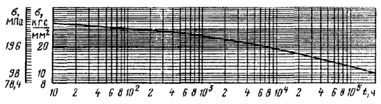
Fig. P6.1.
Curve of long-term strength of steel grade 15KhM at T = 773 K (500 °C) [R20p0.2
= 235 MPa (24 kgf/mm2); Rm20 = 441
MPa (45 kgf/mm2)]
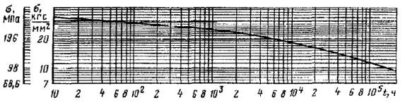
Fig. P6.2.
Curve of long-term strength of steel grade 12KhM at T = 773 K (500 °C) [R20p0.2
= 235 MPa (24 kgf/mm2); R20m
= 441 MPa (45 kgf/mm2)]

Fig. P6.3.
Curve of long-term strength of steels grade 10Kh2M at different temperatures [R20p0.2
= 245 MPa (25 kgf/mm2); R20m =
392 MPa (40 kgf/mm2)]
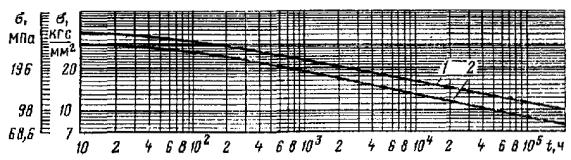
Fig. P6.4.
Curve of long-term strength of steel grade 12Kh2M1:
1 - T = 773 K (500
°C); R20p0.2 = 343 MPa (35
kgf/mm2); R20m = 539 MPa (55
kgf/mm2); 2 - T = 773 K (500 °C); R20p0.2
= 255 MPa (26 kgf/mm2); R20m =
451 MPa (46 kgf/mm2)
when determining the
permissible stresses when selecting the main sizes of components of structures
in accordance with Section 3.2 hereof;
in the calculations of
components of structures for progressive form change, Section 5.10
hereof;
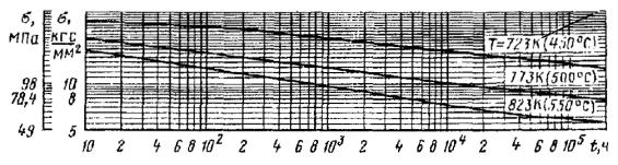
Fig. P6.5.
Curves of long-term strength of steel grade 10Kh2M1FB at different temperatures
[R20p0.2 = 196 MPa (20 kgf/mm2);
R20m = 343 MPa (35 kgf/mm2)]
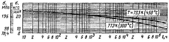
Fig. P6.6.
Curves of long-term strength of steel grade 12Kh1MF at different temperatures [R20p0.2
= 274 MPa (20 kgf/mm2); R20m =
441 MPa (45 kgf/mm2)]
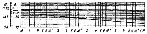
Fig. P6.7.
Curve of long-term strength of steel grade 15Kh1M1F at T = 773 K (500
°C) [R20p0.2 = 314 MPa (32
kgf/mm2); R20m = 490 MPa (50
kgf/mm2)]
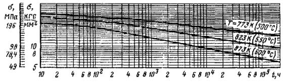
Fig. P6.8.
Curves of long-term strength of steel of grade 12Kh18N9 at different
temperatures [R20p0.2 = 196 MPa
(20 kgf/mm2); R20m = 490 MPa (50
kgf/mm2)]
in calculations for
long-term static and long-term cyclic strength, Section 5.7, 5.9
hereof.
3. EXTRAPOLATION METHOD
FOR LONG-TERM STRENGTH
3.1. The method
is designed to obtain the limits of long-term strength for a given level of
probability of destruction P of structural materials for operating lives
of up to 105 ÷ 2 · 105 h according to the data of experiments
on a long-term rupture of limited (about 104 h) duration.
Implementation of the method is based on determining, at a temperature T1,
of the rupture stress RTmt over time tT1k
under nT1 experiments conducted at a temperature T1,
and nT2 experiments conducted at a temperature T2.
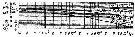
Fig. P6.9.
Curves of long-term strength of steels grade 10Kh18N10T, 12Kh18N12T at
different temperatures [R20p0.2
= 216 MPa (22 kgf/mm2); R20m =
529 MPa (54 kgf/mm2)]
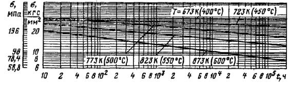
Fig. P6.10.
Curves of long-term strength of steel grade 08Kh16N11M3 at different
temperatures [R20p0.2 = 196 MPa
(20 kgf/mm2); R20m = 510 MPa (52
kgf/mm2)]
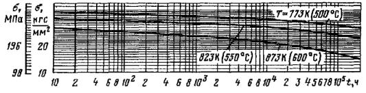
Fig. P6.11.
Curves of long-term strength of alloy grade KhN35VT at different temperatures [R20p0.2
= 392 MPa (40 kgf/mm2); R20m =
736 MPa (75 kgf/mm2)]
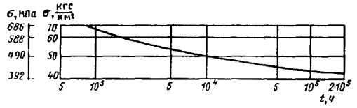
Fig. P6.12.
Curve of long-term strength of alloy grade 1Kh16N36MBTYUR at T = 773 K
(500 °C) [R20p0.2 = 392 MPa (40
kgf/mm2); R20m = 785 MPa (80
kgf/mm2)]
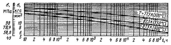
Fig. P6.13.
Curves of long-term strength of steels grades 08Kh18N10T, 10Kh17N13M2T at
different temperatures [R20p0.2
= 196 MPa (20 kgf/mm2); R20m =
510 MPa (52 kgf/mm2)]
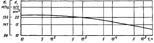
Fig. P6.14.
Curve of long-term strength of steel grade 12Kh18N12M3TL at T = 773 K
(500 °C) [R20p0.2 = 216 MPa (22
kgf/mm2); R20m = 491 MPa (510
kgf/mm2)]
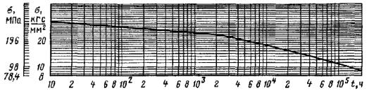
Fig. P6.15.
Curve of long-term strength of steel grade 20KhML at T = 773 K (500 °C)
[R20p0.2 = 245 MPa (25 kgf/mm2);
R20m = 441 MPa (45 kgf/mm2)]
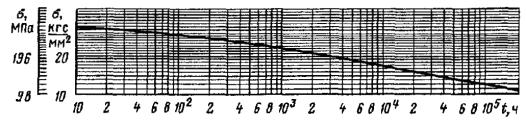
Fig. P6.16.
Curve of long-term strength of steel grade 20KhMFL at T = 773 K (500 °C)
[R20p0.2 = 294 MPa (30 kgf/mm2);
R20m = 490 MPa (50 kgf/mm2)]
When
processing the experimental data (determining the curves of long-term strength
at temperatures T1 and T2), experiments
with a duration of more than 200 hours are used.
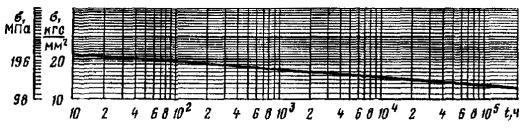
Fig. P6.17.
Curve of long-term strength of steel grade 15Kh1M1FL at T = 773 K (500
°C) [R20p0.2 = 314 MPa (32
kgf/mm2); R20m = 490 MPa (50
kgf/mm2)]
3.2. Dependence
of the rupture stress  on time
  at
temperature Tj (j = 1, 2) is described by the equation
at
temperature Tj (j = 1, 2) is described by the equation
 (P6.1)
where  are constant
coefficients.
are constant
coefficients.
3.3. To clarify
the essence of the method and adopted symbols, Fig. P6.30 gives the way
of its graphic implementation.
Results of
long-term strength tests at temperatures T1 and T2
in Fig. P6.30 are shown as points in the standard coordinate system lgσ
- lgt.
3.4. According
to the experimental points, mean lines of long-term strength at temperatures T1
and T2 are plotted which in accordance with (P6.1) are
generally shown as curvilinear segments. Curve 1 (Fig. P6.30)
corresponds to the test temperature T1, curve 2 – T2.
3.5. For the
maximum test time  at a
temperature T1, curve 1 determines the stress
at a
temperature T1, curve 1 determines the stress  and curve 2
determines time
and curve 2
determines time  corresponding
to this stress.
corresponding
to this stress.
3.6.
Extrapolated long-term strength curve at a temperature T1 and
stresses, lower that  , is obtained by
transferring the curve at T2 to the right over a distance
, is obtained by
transferring the curve at T2 to the right over a distance  . Provided
that
. Provided
that
 (P6.2)
3.7. In
accordance with (P6.2), the limit of long-term strength at a temperature
T1 and given time  is determined by curve
2 at an equivalent time teq. Provided that
is determined by curve
2 at an equivalent time teq. Provided that

3.8. All calculations
according to this extrapolation method are carried out in the following
sequence: determination of the coefficients of equation (P6.1) using
standard procedures of the least squares method; calculation of the
extrapolation coefficient γl-t.s by the formula (P6.2), of
the time  from
equation
from
equation
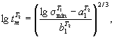 (P6.3)
determination of the
extrapolated long-term strength limit at a temperature T1 and
given operation life  by the formula
 (P6.4)
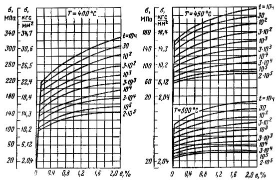
Fig. P6.18.
Isochronous creep curves for steel grade 09G2S at different temperature [R20p0.2
= 245 MPa (25 kgf/mm2); Rm20 = 432 MPa
(44 kgf/mm2): σ0.01/σ0.5 = 0.67]
3.9. Values of
the extrapolated long-term strength limit  at a temperature T1
for a given probability of fracture P are calculated by the formula
at a temperature T1
for a given probability of fracture P are calculated by the formula
 (P6.5)
where ZP
is a quantile of PP level of standard normal distribution determined
according to Table P6.5.
Table P6.5. Value
of coefficient ZP at different values of the fracture probability
P
|
P
|
0.010
|
0.025
|
0.050
|
0.100
|
0.5
|
|
ZP
|
-2.33
|
-1.96
|
-1.64
|
-1.28
|
0.00
|
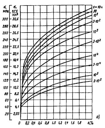
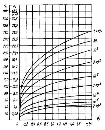
Fig. P6.19.
Isochronous creep curves for steels grades 15KhM and 12KhM [R20p0.2
= 245 MPa (25 kgf/mm2); Rm20 = 441 MPa
(45 kgf/mm2); σ0.01/σ0.5 = 0.80]:
a – at T
= 773 K (500 °C); b – at T = 823 K (550 °C)
Sample
standard deviation Sσ is calculated by the formula
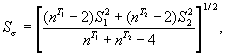 (P6.6)
where
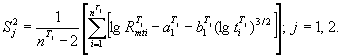 (P6.7)
It is
recommended that the minimum (normative) value of the long-term strength limit
be determined for the probability of fracture P = 0.01.
4.
EXTRAPOLATION METHOD FOR CONDITIONAL LIMITS OF CREEP
4.1. Prediction of creep curves can be made on the basis of
extrapolation of creep limits using the procedures used in the method of
extrapolation of long-term strength according to Section 3.
4.2. Equation to
approximate conditional creep limit curves at temperature Tj
(j = 1, 2) has the form of
 (P6.8)
where  are
coefficients.
are
coefficients.
Conditional
creep limits are determined by replacing the long-term strength limit by the
conditional creep limit in equations (P6.1) - (P6.7), the time to
failure by the time to achieve a given deformation Az, γl-t.s
- γs, and the coefficient γs is determined by the maximum
time to reach a given deformation of Az using procedures similar
to those described for the method of long-term strength in Section 3.
4.3. To predict
creep limits, creep tests for each metal batch are carried out at temperatures T1
and T2 = T1 + 50 K (°C) (see Section 2.8).
According to
the creep test results, deformation curves (primary creep curves) are plotted
in e-t coordinates in accordance with GOST 3248-81. To obtain the
centerline of the steady-state creep, it is recommended to process the creep
curves using the least squares method, assuming y = e as a random
value and x = tz as an independent value.
Using creep
curve, tz corresponding to the specified residual elongation
is found.
4.4. If it is
necessary to obtain isochronous creep curves, it is recommended that the stress
level for each order in time be set equal to 0.85; 0.7; 0.55 σTmin
according to the results of tests for the long-term strength of this batch of
metal.
Isochronous
creep curves (σ - e) are plotted by the parameter t over duration
of 10, 30, 102, 3 · 102, 103, 3 · 103,
104, 3 · 104, 105, 2 · 105 h.
4.5. For each
batch of metal tested at temperatures T1 and T2,
creep curves are plotted in coordinates lgtz - lgσ, which are
used to determine the conditional creep limit by the method of extrapolation
described in Section 3.
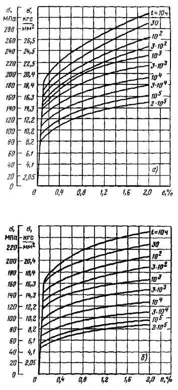
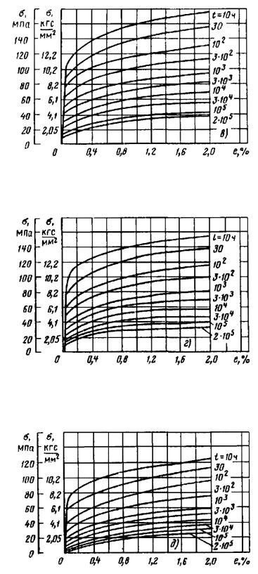
Fig. P6.20.
Isochronous creep curves for steel grade 12Kh2M [R20p0.2
= 245 MPa (25 kgf/mm2); Rm20 = 392 MPa
(40 kgf/mm2); σ0.01/σ0.5 = 0.8]:
a –T =
723 K (450 °C); b – at T = 773 K (500 °C); c – at T
= 823 K (550 °C); d – at T = 838 K (565 °C); e – at T
= 873 K (600 °C)
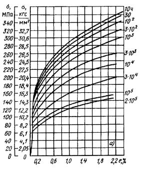
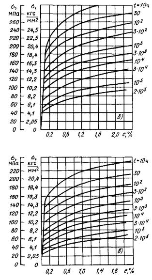
Fig. P6.21.
Isochronous creep curves for steel grade 15Kh1M1F [R20p0.2
= 314 MPa
(32 kgf/mm2); Rm20 = 490 MPa (50 kgf/mm2):
a – at T
= 773 K (500 °C); b – at T = 813 K (540 °C); c – at T
= 843 K (570 °C)
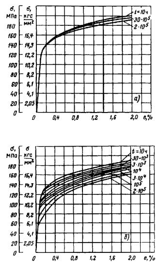
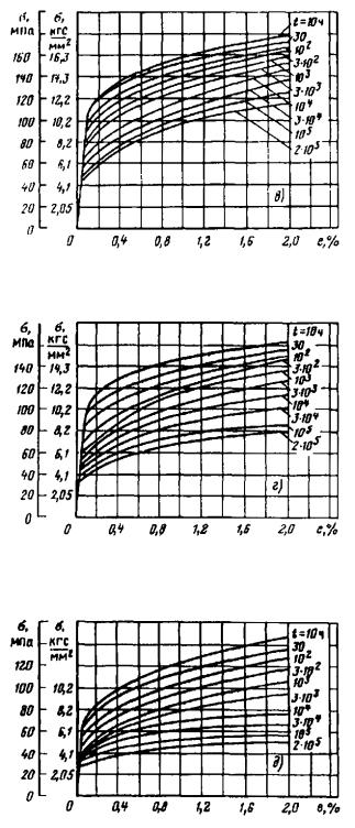
Fig. P6.22.
Isochronous creep curves for steel grade 12Kh18N9 [R20p0.2
= 196 MPa (20 kgf/mm2); Rm20 = 490 MPa
(50 kgf/mm2)]:
a – at T
= 723 K (450 °C); b – at T = 773 K (500 °C); c – at T
= 823 K (550 °C); d – at T = 873 K (600 °C); e – at T
= 923 K (650 °C)
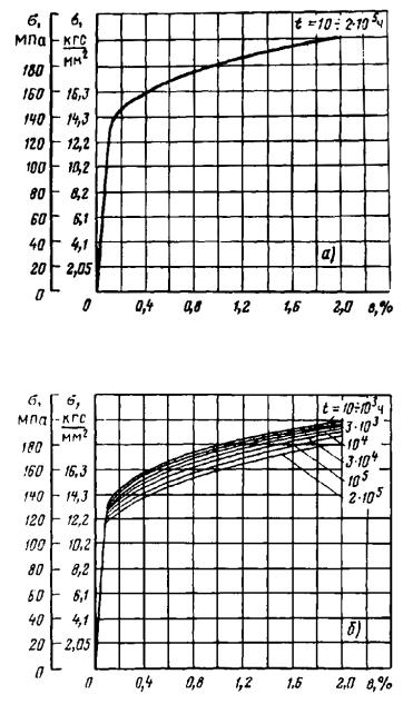
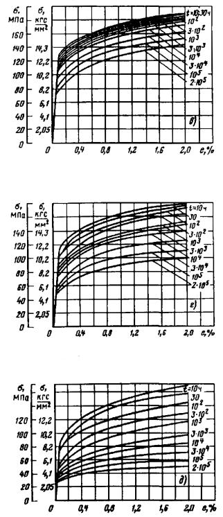
Fig. P6.23.
Isochronous creep curves for steels grades 08Kh16N11M3, 08Kh16N9M2, 12Kh18N12T,
12Kh18N10T [R20p0.2 = 196 MPa
(20 kgf/mm2); Rm20 = 510 MPa (52 kgf/mm2)]:
a – at T
= 723 K (450 °C); b – at T = 773 K (500 °C); c – at T
= 823 K (550 °C); d – at T = 873 K (600 °C); e – at T
= 923 K (650 °C)
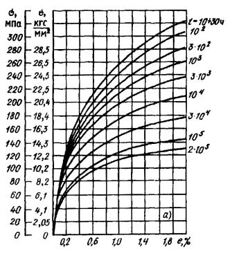
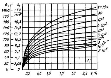
Fig. P6.24.
Isochronous creep curves for steel grade 12Kh1MF: [R20p0.2
= 274 MPa (28 kgf/mm2); Rm20 = 441 MPa
(45 kgf/mm2); σ0.01/σ0.5 = 0.73]:
a – at T
= 773 K (500 °C); b – at T = 823 K (550 °C)
5.
EXTRAPOLATION METHOD FOR CONDITIONAL LIMITS OF STRESS RUPTURE DUCTILITY
5.1. To obtain
the stress rupture ductility characteristics, samples are tested for long-term
strength at temperatures T1 (see Section 2.8) and T2
provided that T2 – T1 ≈ 50 K (°C).
Measurements
of the relative residual elongation and contraction are carried out according
to GOST 10145-81. The test results are processed in coordinates 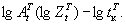
5.2. The
proposed extrapolation method is designed to determine, at a temperature T1,
the stress rupture ductility characteristics  for a given
operation life based on
for a given
operation life based on  experiments
at temperature T1 and
experiments
at temperature T1 and  experiments at
temperature T2.
experiments at
temperature T2.
5.3. Dependence
of residual elongation on time is described by the equations
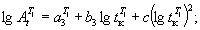 (P6.9)
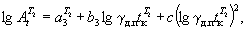 (P6.10)
where  ,
,  , b
and c are constant coefficients; extrapolation coefficient γl-t.s
is determined by the formula (P6.2). Similar equations are accepted for
residual contraction.
, b
and c are constant coefficients; extrapolation coefficient γl-t.s
is determined by the formula (P6.2). Similar equations are accepted for
residual contraction.
5.4. To clarify
the idea of the method, Fig. P6.31 gives the way of its graphic
implementation. This Fig., in coordinates  , shows test results at
temperatures T1 and T2 as dots. When
extrapolating stress rupture ductility curves, experimental points at
temperature T2 are transferred to the right at a distance lgγl-t.s
and equidistant parabolas 1 and 2 are drawn through the obtained and
experimental points at temperature T1. Dotted part of line 1
is the result of extrapolation.
, shows test results at
temperatures T1 and T2 as dots. When
extrapolating stress rupture ductility curves, experimental points at
temperature T2 are transferred to the right at a distance lgγl-t.s
and equidistant parabolas 1 and 2 are drawn through the obtained and
experimental points at temperature T1. Dotted part of line 1
is the result of extrapolation.
5.5.
Coefficients of equations (P6.9) and (P6.10) are determined by
the least square method.
5.6. For a given
operation life tz and temperature T1,
conditional limit of residual elongation  with probability of
fracture P is determined by the formula
with probability of
fracture P is determined by the formula
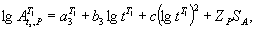 (P6.11)
Values ZP
for different levels of P are given in Table P6.5.
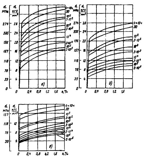
Fig. P6.25.
Isochronous curves for steel grade 05Kh12N2M [R20p0.2
= 372 MPa (38 kgf/mm2); Rm20 = 539 MPa
(55 kgf/mm2)]:
a – at T
= 723 K (450 °C); b – at T = 773 K (500 °C); c – at
T = 823 K (550 °C)
Standard
deviation SA is determined from the equation
SA = (x)1/2
= (α + βη)1/2, (P6.12)
where α and β are
constant coefficients determined by the least square method on the strength of
all the evidence:

cj = 1 at j
= 1; cj = γl-t.s at j = 2.
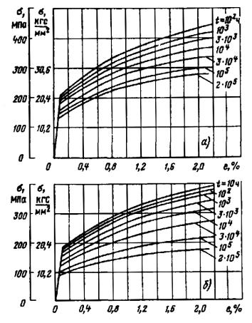
Fig. P6.26.
Isochronous creep curves for steel grade 16GNMA [R20p0.2
= 323 MPa (33 kgf/mm2); Rm20 = 493 MPa
(50 kgf/mm2)]:
a – at T
= 673 K (400 °C); b – at T = 723 K (450 °C)
APPENDIX 7
(recommended)
CALCULATION FOR LONG-TERM CYCLIC STRENGTH
1. The method
of calculation for long-term cyclic strength for isothermal and non-isothermal
loading is applicable in the temperature range from Tt (see
Section 3.2 hereof) to 773 K (500 °C) for parts made of alloy steels,
from 873 K (600 °C) for parts made of corrosion-resistant austenitic steels and
iron-nickel alloys, and to 623 K (350 °C) for parts made of zirconium alloys
with 1 and 2.5% of niobium with the number of cycles of up to 107.
2. The
provisions set forth in Section 5.3 and items 5.6.2, 5.6.3,
5.6.8, 5.6.16 - 5.6.21, 5.6.23 hereof shall be
applied when calculating the long-term cyclic strength.
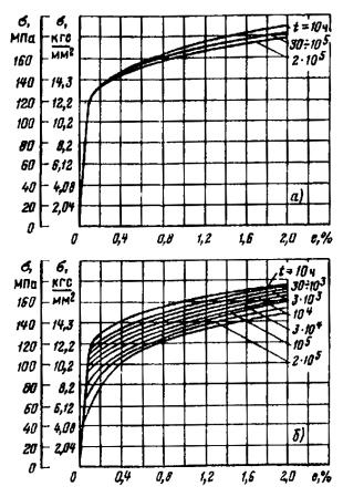
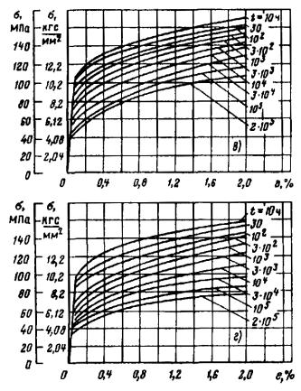
Fig. P6.27.
Isochronous creep curves for steel grade 08Kh18N9 [R20p0.2
= 196 MPa (20 kgf/mm2); Rm20 = 490 MPa
(50 kgf/mm2)]:
a – at T
= 723 K (450 °C); b – at T = 773 K (500 °C); c – at T
= 823 K (550 °C); d – at T = 873 K (600 °C)
3. The
definition of permissible amplitude of conditional elastic stresses or
permissible number of cycles shall be carried out according to the formulas in
item 5.6.6 hereof. Provided that, it shall be assumed
RcT = RTmt(1
– ZTt)-1; ecT
= eTmt; RT-1 = RT-1t;
m = 0.5; me = 0.132lg{2.5[1 – ZtT]-1},
where RTmt
is a limit of long-term strength at maximum load cycle temperature over time t,
equal to the part of the working life of the considered part, worked at a
temperature above Tt (see Section 3.2 hereof); RT-1
is an endurance limit at maximum temperature of cycle and 107 load
cycles over time t, assumed equal to 0.4 RTmt;
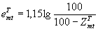 is a
stress rupture ductility characteristic determined by a uniform contraction of
the cross-section ZTmt when long-term static
tension; value of eTmt is assumed minimum in the
range of operating temperatures and duration of load of up to t.
is a
stress rupture ductility characteristic determined by a uniform contraction of
the cross-section ZTmt when long-term static
tension; value of eTmt is assumed minimum in the
range of operating temperatures and duration of load of up to t.
If it is
experimentally justified that RT-1t >
0.4RTmt, then the exponent me is
calculated by the formula me = 0.132lgRTmt/[RT-1t(1
– ZtT)]. The value of RTmt
is assumed according to Table P6.1. The value of ZTmt
is allowed to be determined by the formula ZTmt = ATt/(100
+ ATt), where ATt is
a relative elongation of the sample during long-term static fracture in the
range of operating temperatures and duration of load of up to t; at ATt
≤ 30 %, it is allowed to apply the formula eTmt =
5 · 10-3ATt. The value of ATt
and ZTt is assumed according to Table P6.3.
It is allowed to determine me and Rc by the
formulas
me = 0.132lgRTmt/[RT-1t(1
– ZmtT)]; Rc = RTmt/(1
– ZTmt).
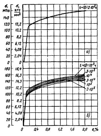
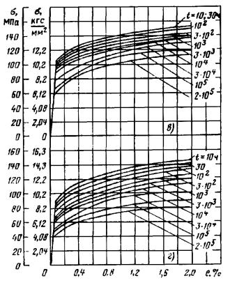
Fig. P6.28.
Isochronous creep curves for steel grade 08Kh18N12T [R20p0.2
= 196 MPa (20 kgf/mm2); Rm20 = 490 MPa
(50 kgf/mm2)]:
a – at T
= 723 K (450 °C); b – at T = 773 K (500 °C); c – at T
= 823 K (550 °C); d – at T = 873 K (600 °C)
4. In the
temperature range of 623 - 673 K (350 - 400 °C) for alloyed steels, 723 - 773 K
(450 - 500 °C) for corrosion-resistant austenitic steels and 523 - 573 K (250 -
300 ° C) for zirconium alloys, eTmt values for
intermediate temperatures are determined by linear interpolation between the
values of eTc and eTmt
at the lowest and highest temperatures of the ranges, respectively. For the
minimum temperatures of these ranges, the value of eTmt
is equal to eTc, which is determined according to
item 5.6.6 hereof.
5. The design
fatigue curves for alloyed steels with a symmetric cycle are shown in Fig. P7.1.
The modulus of elasticity is assumed as 184, 182, 180, 176, 172 GPa at 623,
648, 673, 723 and 773 K (350, 375, 400, 450, 500 °C), respectively. Mechanical
properties when using curves shall be as follows:
up to 623 K (350 °C) R20p0.2/Rm20
≤ 0.7; RTm ≥ 450 MPa; ZT ≥ 32 %;
for t ≤ 2 · 105
h:
up to 673 K (400 °C) RTmt
≥ 195 MPa, AtT ≥ 16 %;
up to 723 K (450 °C) RTmt
≥ 180 MPa, ATt ≥ 15 %;
up to 773 K (500 °C) RTmt
≥ 95 MPa, ATt ≥ 16 %;
The design
fatigue curves for austenitic steels with a symmetric cycle are shown in Fig. P7.2.
The modulus of elasticity is assumed to be 155, 152, 146, 147, 145 GPa at 723,
748, 773, 823, 873 K (450, 475, 500, 550, 600 °C), respectively.
Mechanical
properties when using curves shall be as follows:
up to 723 K (450 °C) R20p0.2/Rm20
≤ 0.7, RTm ≥ 350 MPa, ZT ≥ 45 %;
for t ≤ 2 · 105
h:
up to 773 K (500 °C) RTmt
≥ 166 MPa, ATt ≥ 10 %;
up to 823 K (550 °C) RTmt
≥ 117 MPa, ATt ≥ 16 %;
up to 873 K (600 °C) RTmt
≥ 107 MPa, ATt ≥ 10 %.
The design
fatigue curves for iron-nickel age-hardening alloy KhN35VT with a symmetric
cycle are shown in Fig. P7.3. The modulus of elasticity is assumed to be
163, 162, 161, 158, 156 GPa at 723, 748, 773, 823, 873 K (450, 475, 500, 550,
600 °C), respectively.
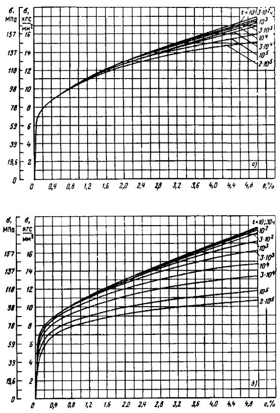

Fig. P6.29.
Isochronous creep curves for steel grade 03Kh16N9M2 [R20p0.2
= 200 MPa (21 kgf/mm2); Rm20 = 520
MPa (53 kgf/mm2)]:
a – at T
= 773 K (500 °C); b – at T = 823 K (550° C); c – at T
= 873 K (600 °C); d – at
T = 923 K (650о C)
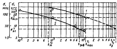
Fig. P6.30.
Graph of long-term strength:
1 – tests at T1;
2 – tests at T2
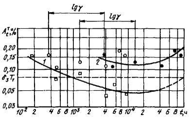
Fig. P6.31.
Graph of residual elongation limits:
1 – tests at T1
(□); 2 – tests at T2  , after
recalculation
, after
recalculation 
Mechanical
properties when using curves shall be as follows:
up to 723 K (450 °C) R20p0.2/Rm20
≤ 0.7; RTm ≥ 620 MPa; ZT ≥ 24 %;
at t ≤ 2 · 105
h;
up to 773 K (500 °C) RTmt
≥ 240 MPa, ATt ≥ 3 %;
up to 823 K (550 °C) RTmt
≥ 210 MPa, ATt ≥ 3 %;
up to 873 K (600 °C) RTmt
≥ 115 MPa, ATt ≥ 4 %.
Fig. P7.1. Design fatigue
curves for alloyed steels when duration of load of 2 · 105 h
|
МПа
|
MPa
|
|
число циклов
|
Number of cycles
|
Fig. P7.2.
Design fatigue curves for corrosion-resistant austenitic steels
when duration of load of 2 · 105 h
Design fatigue
curves for zirconium alloy with 2.5% of niobium with a symmetric cycle are
shown in Fig. P7.4. The modulus of elasticity is assumed to be 75, 72,
69 GPa at temperatures of 523, 573, 623 K (250, 300, 350 °C), respectively.
Mechanical
properties when using curves shall be as follows:
up to 523 K (250 °C) RTm
≥ 335 MPa; ZT ≥ 57 %;
for t ≤ 2 · 105
h:
up to 573 K (300 °C) RTmt
≥ 205 MPa, ATt ≥ 22 %;
up to 623 K (350 °C) RTm
≥ 140 MPa, ATt ≥ 24 %.
When
determining the design curves in Fig. P7.1 - P7.4 it is assumed
that nσ = 2 and nN = 10.
Design curves
for intermediate temperatures can be obtained by interpolation of stresses.
Fig. P7.3. The
design fatigue curves for the iron-nickel age-hardening alloys (KhN35VT) with a
duration of load of 2 · 105 h
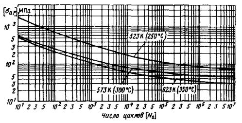
Fig. P7.4.
Design fatigue curves of a zirconium alloy with 2.5% Nb
with a duration of load of 2 · 105 h
6. When
calculating components of structures made of homogeneous materials or their
zones loaded only with temperature stresses from radial temperature differences
(excluding zones of edge effect and changes in mean temperature); for example,
heat, screens, separation shells, etc., the fracture of which does not result
in the medium leaving the supporting components that hold it, as well as mixing
sodium with an aqueous medium, safety factors when calculating these components
or their zones for long-term cyclic strength in according to items 3 - 5 of
this Appendix and formulas of item 5.6.6 hereof are assumed equal to nσ
= 1.5 and nN = 5.
7. If when
calculation according to items 2 - 5 of this Appendix the conditions of
strength or applicability of curves are not satisfied, then the specification
of the permissible number of cycles or permissible amplitudes of local stresses
obtained from the calculated fatigue curves or formulas can be carried out
according to the formulas of item 5.6.6 hereof and items 3, 4 of this
Appendix on the basis of an analysis of the process of change of temperatures
and stresses in the zone under consideration in accordance with the following
items.
8. If the
loading during operation is performed at different temperatures, then the RTmt
and eTmt values can be determined with due regard
to the non-stationarity of the thermal mode. The value of RTmt
= (RTmt)pr is assumed according to the
curve of long-term strength at maximum temperature (Tσ)0
of cycle for duration of load (tσ)pr ≤ t0:
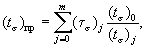
where (τσ)j
is a total loading time at temperature (Tσ)j;
(tσ)j is time to fracture along the curve
of long-term static strength at temperature (Tσj) at stress (RTmt)
causing fracture at temperature (Tσ)0 over time (tσ)0.
In a similar
way, the value of eTmt is determined. To obtain (te)pr,
a change curve is used eTmt at temperature (Te)0
leading to the greatest loss of ductility during long-term static load. The
value of eTmt = (eTmt)pr
is assumed according to the curve of its change depending on the time to
long-term static fracture at a temperature (Te)0
for duration of load (te)pr ≤ t0
(in general case (tσ)pr ≠ (te)pr:
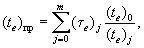
where (τe)j
is a general loading time at temperature (Te)j;
(te)j is time to reach, according to the
change curve eTmt at temperature (Te)j,
values of (eTmt)0, corresponding to the
temperature (Te)0 and time (te)0.
If the values
of eTmt reach the minimum at some time before
fracture t', then at t > t' the value of eTmt
is assumed to be the minimum.
The values of
(RTmt)pr and (eTmt)pr
are used to calculate [N0] and [σaF] by the
formulas in item 5.6.6 hereof and items 3, 4 of this Appendix.
Fig. P7.5
and P7.6 give examples of the definition (RTmt)pr
and (eTmt)pr. Shows the case of two
operating temperatures leading to temperature (Tσ)0
when determining (tσ)pr and temperature, leading
to the greatest loss of ductility when determining (te)pr.
9. If when
calculation according to items 2 - 8 of this Appendix, the strength condition
is not satisfied, then in order to clarify the result obtained, the design time
for the cycle in question is assumed to be the greatest of (tσ)pr
and (te)pr.
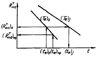
Fig. P7.5. The
scheme of accounting the non-stationarity of thermal mode in determining the
reduced limit of long-term strength
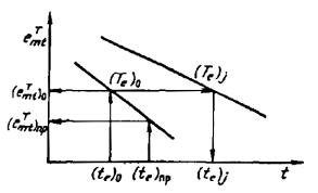
Fig. P7.6. The
scheme of accounting the non-stationarity of thermal mode in determining the
reduced value of stress rupture ductility
The longest
time specified, for example (te)pr, is divided
into time intervals for which the expected operational number of cycles of this
type is known, and for moments of time corresponding to the end of intervals,
is selected according to the curve of long-term strength at temperature (Tσ)0
and curve of changes eTvt at temperature (Te)0
of values of RTmt and eTmt
(Fig. P7.7).
According to
the formula of item 5.6.6 hereof and items 3, 4 of this Appendix the
calculation of the permissible number of cycles [N0] of this
type is carried out characterized by stress amplitude (σaF)
and asymmetry r using RTmt and eTmt
values corresponding to the accepted division of duration of load into
intervals.
The total
fatigue damage, with due regard to damages from other types of cycles, shall
satisfy the condition of item 5.6.19 hereof.
10. If when
calculation according to items 8, 9 of this Appendix, the value of eTmt
does not change over time and is determined only by temperature, then the
loading time t shall be divided into separate intervals corresponding to
different temperatures of the cycle under consideration; within these
intervals, for which the expected operational number of cycles is known, the
calculation of the permissible number of cycles [N0] of this
type, characterized by stress amplitude (σaF) and asymmetry
coefficient r, is carried out according to the formulas of item 5.6.6
hereof and items 3, 4 of this Appendix, using the values of RTmt
and eTmt, corresponding to the duration of
intervals and temperature values within these intervals.
The total
fatigue damage, with due regard to damages from other types of cycles, shall
satisfy the condition of item 5.6.19 hereof.
11. In the case
when deformations and stresses are obtained from the calculation with due
regard to creep, the values of RTmt and eTmt
can be determined by the actual level of long-term static fractures. For this
purpose, long-term static fractures Dt, accumulated during
operational loading, are calculated. Operational loading includes all types of
cycles with the number of repetitions equal to the expected for the service
life of the part, and reflects the actual mean duration of loading for each
type of cycle and the corresponding temperatures in the part zone in question.
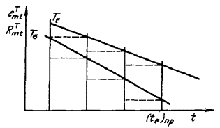
Fig. P7.7.
Scheme of accounting the dependence of the limit of long-term strength and
long-term ductility over time
Long-term
static fracture

where t is time
to fracture under long-term static loading by the actual reduced local stress
at the corresponding temperature in the zone of part being considered.
This equally
takes into account the fractures from tension and compression stresses if for
these values of temperatures and stresses the absence of fractures from
compression stresses or their smaller value compared to tension was not
experimentally shown.
The values of RTmt
and eTmt when assessing long-term cyclic strength
according to item 5.6.6 hereof and items 3, 4 of this Appendix are
assumed according to the curve of long-term strength at the maximum temperature
of the cycle and according to curve of change eTmt
depending on the time at the temperature of the loading cycle, leading to the
greatest reduction in ductility, for duration of load t* = Dtt.
Long-term static fracture shall satisfy the condition Dt ≤ 1.
At Dt = 1 time t* is t. Under
non-stationary load (presence of several types of cycles), the strength
condition shall be satisfied in accordance with item 5.6.19 hereof.
Clarification
of the calculation under this item can be carried out in the same manner as
indicated in item 1.9 of this Appendix.
12. When using
steels with a content of non-metallic inclusions above the 3rd grade determined
according to GOST 1778-70, the permissible number of cycles of this type shall
be determined from the design fatigue curves of items 3 - 5 of this Appendix with
stress amplitude.
(σaF)
= (σaF) + KFv∆α∆TET,
where (σaF)
is a design amplitude of the reduced elastic stresses from mechanical and
thermal loads;
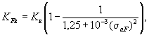
where Kv
is a coefficient of influence of non-metallic inclusions assumed from Table P7.1;
∆α is an absolute value of the difference between the coefficients of thermal
expansion of steel and non-metallic inclusions according to Table P7.1;
∆T is a cycle temperature range determined by the formula
∆T = Tmax
– Tmin,
where Tmax
and Tmin are maximum and minimum temperatures of cycle of
stresses.
Table P7.1. Values
of Kv and ∆α
|
Material
|
Level of
pollution, points
|
Kv
|
∆α, 10-6
1/°C
|
|
Sheet
|
Rod, pipe
blank
|
Forging
|
|
350 °С
|
400 °С
|
450 °С
|
500 °С
|
550 °С
|
600 °С
|
350 °С
|
400 °С
|
450 °С
|
500 °С
|
550 °С
|
600 °С
|
350 °С
|
400 °С
|
450 °С
|
500 °С
|
550 °С
|
600 °С
|
|
Alloy steels and
welded joints
|
3.0
|
0
|
0
|
0
|
0
|
0
|
-
|
0
|
0
|
0
|
0
|
0
|
-
|
0
|
0
|
0
|
0
|
0
|
-
|
7
|
|
3.5
|
0
|
0.04
|
0.07
|
0.11
|
0.14
|
-
|
0
|
0.025
|
0.05
|
0.08
|
0.10
|
-
|
0
|
0.02
|
0.04
|
0.06
|
0.08
|
-
|
|
4.0
|
0
|
0.04
|
0.08
|
0.12
|
0.16
|
-
|
0
|
0.03
|
0.06
|
0.09
|
0.12
|
-
|
0
|
0.02
|
0.045
|
0.065
|
0.09
|
-
|
|
4.5
|
0
|
0.045
|
0.09
|
0.14
|
0.18
|
-
|
0
|
0.035
|
0.07
|
0.11
|
0.14
|
-
|
0
|
0.025
|
0.05
|
0.08
|
0.10
|
-
|
|
5.0
|
0
|
0.05
|
0.10
|
0.15
|
0.20
|
-
|
0
|
0.04
|
0.08
|
0.12
|
0.16
|
-
|
0
|
0.03
|
0.06
|
0.09
|
0.12
|
-
|
|
Austenitic steel and
welded joints
|
3.0
|
-
|
-
|
0
|
0
|
0
|
0
|
-
|
-
|
0
|
0
|
0
|
0
|
-
|
-
|
0
|
0
|
0
|
0
|
10
|
|
3.5
|
-
|
-
|
0
|
0.07
|
0.14
|
0.20
|
-
|
-
|
0
|
0.05
|
0.11
|
0.16
|
-
|
-
|
0
|
0.04
|
0.08
|
0.12
|
|
4.0
|
-
|
-
|
0
|
0.08
|
0.16
|
0.24
|
-
|
-
|
0
|
0.06
|
0.12
|
0.18
|
-
|
-
|
0
|
0.045
|
0.09
|
0.14
|
|
4.5
|
-
|
-
|
0
|
0.09
|
0.18
|
0.28
|
-
|
-
|
0
|
0.07
|
0.14
|
0.22
|
-
|
-
|
0
|
0.05
|
0.11
|
0.16
|
|
5.0
|
-
|
-
|
0
|
0.10
|
0.20
|
0.30
|
-
|
-
|
0
|
0.08
|
0.16
|
0.24
|
-
|
-
|
0
|
0.06
|
0.12
|
0.18
|
|
Iron-nickel
age-hardening alloys and welded joints
|
3.0
|
-
|
-
|
0
|
0
|
0
|
0
|
-
|
-
|
0
|
0
|
0
|
0
|
-
|
-
|
0
|
0
|
0
|
0
|
8
|
|
3.5
|
-
|
-
|
0
|
0.07
|
0.14
|
0.20
|
-
|
-
|
0
|
0.05
|
0.11
|
0.16
|
-
|
-
|
0
|
0.04
|
0.08
|
0.12
|
|
4.0
|
-
|
-
|
0
|
0.08
|
0.16
|
0.24
|
-
|
-
|
0
|
0.06
|
0.12
|
0.18
|
-
|
-
|
0
|
0.045
|
0.09
|
0.14
|
|
4.5
|
-
|
-
|
0
|
0.09
|
0.18
|
0.28
|
-
|
-
|
0
|
0.07
|
0.14
|
0.22
|
-
|
-
|
0
|
0.05
|
0.11
|
0.16
|
|
5.0
|
-
|
-
|
0
|
0.10
|
0.20
|
0.30
|
-
|
-
|
0
|
0.08
|
0.16
|
0.24
|
-
|
-
|
0
|
0.06
|
0.12
|
0.18
|
13. In the
absence of data on the content of non-metallic inclusions, the calculation of
the permissible number of cycles shall be carried out according to item 12
assuming the value of coefficient Kv for the 5th grade.
14. When
calculating the long-term cyclic strength of welded joints, the rated stress
amplitude is determined as
(σaF)s
= (σaF)v/φs,
where φs
is a coefficient of reducing the long-term cyclic strength of the welded joint,
assumed from Table P7.2 depending on the maximum temperature of the
cycle.
15. When
calculating the cyclic strength of components of structures operating in
contact with a reactor-grade corrosion-active medium, the permissible number of
cycles is determined according to the design fatigue curve of items 3 - 5 of
this Appendix and the formulas of items 5.6.6 and 5.6.7 hereof
(at moderately elevated temperatures that do not cause creep) for the stress
amplitude determined by the formula
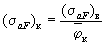
or
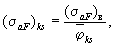
where (σaF)v
is an amplitude of the conditional elastic stress, determined according to
items 12, 13 of this Appendix and Section 5.3 hereof;  and
and  are
coefficients of corrosion reduction of the cyclic strength of the base metal
and welded joint, determined in accordance with the requirements of item 9.6
of Appendix 2 hereof.
are
coefficients of corrosion reduction of the cyclic strength of the base metal
and welded joint, determined in accordance with the requirements of item 9.6
of Appendix 2 hereof.
Table P7.2. Values
of coefficients φs
|
Base
metal
|
Welding
technique
|
Welding
material
|
Types of
heat treatment after welding
|
Temperature,
°С
|
|
350
|
400
|
450
|
500
|
550
|
600
|
|
Austenitic steels
|
Manual
|
48A-1
|
Without heat treatment
|
-
|
-
|
0.8
|
0.70
|
0.60
|
0.50
|
|
Austenitization
|
-
|
-
|
1.0
|
0.85
|
0.70
|
0.55
|
|
48A-2-VI
|
Without heat treatment
|
-
|
-
|
0.8
|
0.70
|
0.60
|
0.55
|
|
Austenitization
|
-
|
-
|
0.8
|
0.70
|
0.55
|
0.45
|
|
EA400/10u
|
Without heat treatment
|
-
|
-
|
0.8
|
0.70
|
0.60
|
0.50
|
|
Austenitization
|
-
|
-
|
0.8
|
0.70
|
0.60
|
0.55
|
|
Argonarc
|
Sv-04Kh17N10M2
|
Without heat treatment
|
-
|
-
|
0.9
|
0.80
|
0.70
|
0.60
|
|
Austenitization
|
-
|
-
|
1.0
|
0.90
|
0.75
|
0.65
|
|
Sv-02Kh17N10M2-VI
|
Without heat treatment
|
-
|
-
|
0.9
|
0.80
|
0.70
|
0.65
|
|
Austenitization
|
-
|
-
|
0.9
|
0.80
|
0.65
|
0.55
|
|
Sv-04Kh19N11M3
|
Without heat treatment
|
-
|
-
|
1.0
|
0.85
|
0.70
|
0.55
|
|
Austenitization
|
-
|
-
|
1.0
|
0.85
|
0.70
|
0.60
|
|
EP-198
|
Without heat treatment
|
-
|
-
|
0.5
|
0.45
|
0.40
|
0.40
|
|
Austenitization
|
-
|
-
|
0.5
|
0.50
|
0.45
|
0.45
|
|
Automatic
|
Sv-04Kh17N10M2
|
Without heat treatment
|
-
|
-
|
0.8
|
0.70
|
0.55
|
0.45
|
|
Austenitization
|
-
|
-
|
1.0
|
|
|
|
|
Sv-02Kh17N10M2-VI
|
Without heat treatment
|
-
|
-
|
0.8
|
0.70
|
0.60
|
0.50
|
|
Austenitization
|
-
|
-
|
0.8
|
0.70
|
0.55
|
0.45
|
|
Sv-04Kh19N11M3
|
Without heat treatment
|
-
|
-
|
0.8
|
0.70
|
0.60
|
0.50
|
|
Austenitization
|
-
|
-
|
0.8
|
0.70
|
0.60
|
0.55
|
|
Electroslag
|
Sv-04Kh17N10M2
|
Without heat treatment
|
-
|
-
|
0.7
|
0.70
|
0.55
|
0.45
|
|
Austenitization
|
-
|
-
|
1.0
|
0.85
|
0.70
|
0.55
|
|
Sv-04Kh19N11M3
|
Without heat treatment
|
-
|
-
|
0.8
|
0.70
|
0.55
|
0.45
|
|
Austenitization
|
-
|
-
|
0.9
|
0.80
|
0.65
|
0.55
|
|
Iron-nickel
age-hardening alloys
|
Argonarc
|
Sv-Kh15N35
|
Without heat treatment
|
-
|
-
|
0.7
|
0.65
|
0.55
|
0.50
|
|
Austenitization
|
-
|
-
|
0.8
|
0.70
|
0.60
|
0.55
|
|
EP-198
|
Without heat treatment
|
-
|
-
|
0.5
|
0.45
|
0.40
|
0.40
|
|
Austenitization
|
-
|
-
|
0.5
|
0.50
|
0.45
|
0.45
|
|
Steel 12Kh2M
|
Manual
|
48N-10
|
High tempering
|
1.0
|
0.80
|
0.7
|
0.60
|
0.55
|
0.50
|
|
48A-1,
|
Without heat treatment
|
1.0
|
0.85
|
0.7
|
-
|
-
|
-
|
|
EA-395/9
|
High tempering
|
1.0
|
0.80
|
0.6
|
-
|
-
|
-
|
|
48A-1, KTI-7
|
Without heat treatment
|
-
|
-
|
-
|
0.60
|
0.55
|
0.50
|
|
High tempering
|
-
|
-
|
-
|
0.50
|
0.40
|
0.30
|
|
Automatic submerged
|
Sv-04Kh2MA
|
High tempering
|
0.7
|
0.65
|
0.6
|
0.60
|
0.55
|
0.55
|
16. The effect
of contact with reactor-grade sodium or argon is not taken into account when
calculating long-term cyclic strength. It is allowed to increase the
permissible number of cycles for zones of parts operating in contact with
sodium or argon, whose composition satisfies the requirements of operation
guideline for the entire operating life. The permissible number of cycles is
assumed as the minimum of two values:
number of cycles [N0]
determined according to items 1 - 14 of this Appendix and item 5.6.6
hereof for stress amplitude (σaF)v multiplied by a
factor χNa.
[N0]Na
= χNa[N0],
number of cycles
according to the design fatigue curve of items 3-5 of the this Appendix for the
amplitude of the reduced conditional elastic stress (σaF)v
divided by the coefficient φNa.
Values of
coefficients χNa and φNa are given in Table
P7.3.
17. When
calculating the long-term cyclic strength of components of structures operating
under neutron exposure, the permissible number of cycles of this type is
assumed as the minimum of two values:
number of cycles [N0]F
= [N0]/χF, where [N0] is
a number of cycles for the stress amplitude according to items 3 - 16 of this
Appendix or items 5.6.6, 5.6.7 hereof (during calculations for
conditions of moderately elevated temperatures that do not cause creep);
the number of cycles
according to the design fatigue curve or to the corresponding equations for the
stress amplitude determined according to items 3 - 16 of this Appendix or items
5.6.6, 5.6.7 hereof and divided by the coefficient φF.
Values of
coefficients χF and φF are given in Table P7.4.
18. When
determining the permissible number of cycles based on the design fatigue curves
or formulas of item 5.6.6 hereof for parts with surface diffusion chrome-nitride
coating, the stress amplitude (σaF)p is calculated
by the formula
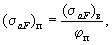
where (σaF)v
is an amplitude of conditional elastic stresses determined according to item 2.17
of this Appendix; φp is a coefficient assumed to be 0.75 for
austenitic steels and iron-nickel age-hardening alloys.
Table P7.3. Values
of coefficients χNa and φNa
|
Material
|
Temperature,
°С
|
Coefficient
|
Load
duration, h
|
|
10
|
102
|
103
|
104
|
105
|
2 · 105
|
|
Alloyed steels
|
20 - 360
|
χNa
|
1
|
1
|
1
|
1
|
1
|
1
|
|
φNa
|
1
|
1
|
1
|
1
|
1
|
1
|
|
400
|
χNa
|
1
|
1
|
1.4
|
1.7
|
2.0
|
2.1
|
|
φNa
|
1
|
1
|
-
|
-
|
-
|
-
|
|
450
|
χNa
|
1
|
1.5
|
2.0
|
2.5
|
3.0
|
3.2
|
|
φNa
|
1
|
-
|
1.05
|
1.05
|
1.05
|
1.05
|
|
500
|
χNa
|
1
|
2.0
|
3.0
|
4.0
|
5.0
|
5.4
|
|
φNa
|
1
|
-
|
1.05
|
1.10
|
1.10
|
1.10
|
|
550
|
χNa
|
1
|
2.5
|
4.0
|
5.5
|
7.0
|
7.5
|
|
φNa
|
1
|
-
|
1.10
|
1.15
|
1.15
|
1.15
|
|
Austenitic steels
|
20 - 450
|
χNa
|
1
|
1
|
1
|
1
|
1
|
1
|
|
φNa
|
1
|
1
|
1
|
1
|
1
|
1
|
|
500
|
χNa
|
1
|
1.5
|
2.0
|
2.5
|
3.0
|
3.2
|
|
φNa
|
1
|
-
|
1.05
|
1.05
|
1.05
|
1.05
|
|
550
|
χNa
|
1
|
2.0
|
3.0
|
4.0
|
5.0
|
5.4
|
|
φNa
|
1
|
-
|
1.05
|
1.10
|
1.10
|
1.10
|
|
600
|
χNa
|
1
|
2.5
|
4.0
|
5.5
|
7.0
|
7.5
|
|
φNa
|
1
|
-
|
1.10
|
1.15
|
1.15
|
1.15
|
|
20 - 450
|
χNa
|
1
|
1
|
1
|
1
|
1
|
1
|
|
φNa
|
1
|
1
|
1
|
1
|
1
|
1
|
|
500
|
χNa
|
1
|
1
|
1.1
|
1.3
|
1.5
|
1.6
|
|
φNa
|
1
|
1
|
-
|
-
|
-
|
-
|
|
Iron-nickel
age-hardening alloys
|
550
|
χNa
|
1
|
1.1
|
1.4
|
1.7
|
2.0
|
2.1
|
|
φNa
|
1
|
1
|
-
|
-
|
-
|
-
|
|
600
|
χNa
|
1
|
1.5
|
2.0
|
2.5
|
3.0
|
3.2
|
|
φNa
|
1
|
-
|
1.05
|
1.05
|
1.05
|
1.05
|
Note. For
intermediate temperatures, the values of coefficients χNa and
φNa are obtained by linear interpolation.
APPENDIX 8
(recommended)
DESIGN AND EXPERIMENTAL METHODS FOR
ASSESSMENT OF VIBRATION STRENGTH OF STANDARD COMPONENTS OF STRUCTURES
1. GENERAL
1.1. This
Appendix to the Regulations contains recommended methods for the calculation
and experimental assessment of parameters of vibration and vibration strength
of equipment and pipelines of nuclear power plants.
1.2. This
Appendix contains the methods for calculating assessment of natural oscillation
frequencies of standard components and the experimental methods for determining
the vibration stress of assemblies on models and full-size components of
structures.
1.3. To assess
the natural oscillation frequencies of equipment components, this Appendix
presents a number of design diagrams relating to the most typical assemblies,
such as pipelines (bar systems), plates and shallow shells.
1.4. To assess
the level of vibrations and vibration stresses in the absence of calculation
procedures and information about the parameters of the existing dynamic loads,
experimental research methods are proposed that are carried out in all modes
provided by the commissioning work program, including the initial stage of
operation of the installations in steady-state modes.
Table P7.4. Values
of coefficients χF and φF
|
Type
of material
|
Temperature,
K (°C)
|
Coefficient
|
FN, m-2
(E ≥ 0.1 MeV)
|
|
1022
|
1023
|
1024
|
1025
|
1026
|
2 · 1026
|
4 · 1026
|
6 · 1026
|
8 · 1026
|
1027
|
|
Alloyed steels
|
293 – 623
(20 - 350)
|
χF
|
1.0
|
2.2
|
5.0
|
-
|
-
|
-
|
-
|
-
|
-
|
-
|
|
Zirconium alloys
|
293 – 623
(20 - 350)
|
φF
|
1.0
|
1.4
|
1.9
|
2.6
|
3.6
|
-
|
-
|
-
|
-
|
-
|
|
Austenitic steels
|
748 – 873
(475 - 600)
|
χF
|
1.0
|
0.90
|
0.85
|
0.80
|
0.75
|
0.7
|
0.67
|
0.65
|
0.63
|
0.6
|
|
293 – 873
(20 - 600)
|
φF
|
1.0
|
1.6
|
2.6
|
4.2
|
6.5
|
10
|
17
|
30
|
-
|
-
|
|
Iron-nickel
age-hardening alloys
|
748 – 873
(475 - 600)
|
χF
|
1.0
|
1.0
|
1.0
|
1.0
|
0.97
|
0.95
|
0.9
|
0.8
|
0.60
|
0.4
|
|
293 – 873
(20 - 600)
|
φF
|
1.0
|
1.0
|
1.0
|
1.0
|
1.2
|
1.4
|
2.0
|
3.6
|
-
|
-
|
Note. For
intermediate neutron transfer values, the coefficients χF and
φF are obtained by linear interpolation.
1.5. As the main
condition for the vibration strength of components of structures, the frequency
detuning of the natural oscillation from frequencies of deterministic
excitation is recommended.
Based on the
experimental data on the vibration-stressed state of the components of structures,
it is proposed to calculate their durability.
1.6. The
following is assumed as a deterministic excitation frequencies:
the main frequency of
the pump shaft speed
ω = 2pn/60,
where n is a
shaft speed, min-1;
the frequency of
electromagnetic forces caused by the presence of slots in the stator and rotor
of drive motors of pumps,

where Zrot
is a number of rotor slots;
the frequency of
hydrodynamic forces determined by the number of blades Z of the pump
impeller,

the frequency of
hydrodynamic forces associated with the breakdown of vortices during the
transverse flow of components of structures by the coolant,

where St is a
dimensionless Strouhal number (for example, for a single rod, it is assumed to
be 0.2, for Reynolds numbers 300 ÷ 5 · 105); v is a flow
rate; d is a characteristic size of a streamlined component in the
cross-section.
1.7. Excitation
associated with the pulsations of pressures and flow rates of coolant, inter
alia arising from the longitudinal and oblique flow around components of
structures, is generally considered as a loading process with a broadband
spectrum having a random character.
In this case,
the vibration strength is assessed by calculating the durability of the
components according to the values of amplitudes of alternating stresses
obtained experimentally on models or full-size structures.
1.8. This
Appendix does not address issues related to abrasion and wear of components
caused by vibrations.
1.9. This
Appendix describes the processes whose parameters remain constant during a
given structure life.
1.10. For complex
cases of calculation of the natural oscillation frequencies of spatial and
branched bar systems, approximate procedures and work programs based on energy
and other methods can be used.
1.11. When
drawing up diagrams (models) for calculating the natural oscillation
frequencies, structural assemblies of reactors and steam generators and
pipelines are presented in the form of simple components, such as bar systems,
plates and shallow shells.
1.12. Pipeline
systems, tubes, solid cylinders, supporting beams of arbitrary cross-section
are considered in the calculations as beams or bar systems with specified
boundary conditions. Heat shields are considered as shallow shells. Plates,
base plates are considered as plates.
1.13. Shut-off
and control valves installed on pipelines and other structural components are
considered in the calculations as lumped masses.
1.14. Calculation
of natural oscillations of the components is carried with due regard to the
added mass of the coolant, but without taking into account its movement,
provided that the flow rate is v ≤ 0.3vkr, where  is a
critical coolant flow rate at which a loss of stability of a rectilinear
hinge-supported component of a pipeline with a span length l occurs; m
is a coolant mass per unit length; EJ is a bending stiffness of the rod.
is a
critical coolant flow rate at which a loss of stability of a rectilinear
hinge-supported component of a pipeline with a span length l occurs; m
is a coolant mass per unit length; EJ is a bending stiffness of the rod.
For example,
when the external flow around a single component, the attached mass is assumed
to be equal to the mass of the displaced fluid.
1.15. Calculation
of the natural frequencies of bending oscillations is carried out without
taking into account the damping of systems.
2. CALCULATION OF NATURAL
OSCILLATION FREQUENCY OF BAR SYSTEMS
2.1. The presented
calculation diagrams refer only to flat bar systems.
2.2. The natural
frequency corresponding to the k-th form of bending oscillations of the
bar systems, with due regard to the coolant mass, is determined by the formula

where Ωk
= 2pfk; fk is a number of oscillations per
1 s; (αl)k is the k-th root of the frequency
equation; l is a rod length between supports; EJ is a bending
stiffness; mc, mt is a mass per unit length
of the rod and the considered coolant, respectively.
2.3. For the
construction of a frequency equation, the general expression of own forms of
bending oscillations is used
X(x) = C1S(αx) + C2T(αx) + C3U(αx) + C4V(αx), (P8.2)
where X(x)
is a function of coordinate x, having the value from 0 to t; C1,
C2, C3, C4 are arbitrary
constants defined by boundary conditions; S(αx), T(αx), U(αx),
V(αx) - tabulated Krylov functions defined by expressions
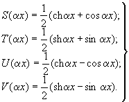 (P8.3)
The following
values are assumed as the boundary conditions in the support cross-sections of
a rod:
deflection X(0, l);
angle of rotation X'(0,
l);
moment EJX"(0,
l);
shear force EJX"(0,
l), where X'(0, l); X"(0, l); X"'(0,
l) - 1-st, 2-nd and 3-rd derived equations (P8.2).
From the
obtained system of four equations, with due regard to (P8.3), the
determinant is composed of the coefficients at the constant C1,
C2, C3 and C4 and equals zero.
Expansion of
the determinant gives a frequency equation whose roots are a set of values (αl)k.
For estimated calculations, we are limited to finding the first two or three
roots (αl) corresponding to the main forms of oscillations. The number
of roots of the frequency equation to be taken into account is determined by
the width of the spectrum of loads that can cause any noticeable vibration.
2.4. For typical
design schemes of bar systems and beams with different conditions of fixing,
Tables P8.1 - P8.3 give the values of the roots of the frequency
equations corresponding to the main forms of oscillations.
Table P8.1
gives the values of the roots of the frequency equations of single-span beams
at different options of fixing. Tables P8.2 and P8.3 contain the
values of the roots of the frequency equation for L-shaped sections of rods
depending on the bend angle ψ to determine the fundamental natural oscillation
frequency in a plane perpendicular to the bend plane.
2.5. In the
calculation of bar systems with a step change in the cross-sections with
intermediate supports and additional masses, when generation of the frequency
equations, the conditions of conjugation of adjacent sections are considered.
Analytical
conjugation conditions are written in the form of: displacement equality Х-
= Х+;
Table P8.1. Values
of αl for rods with different conditions of fixing
|
Scheme
of rod
|
Oscillation
mode number
|
|
1
|
2
|
3
|
4
|
|
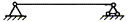
Supported-supported
|
3.142
|
6.283
|
9.425
|
12.566
|
|
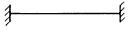
Clamped-clamped
|
4.730
|
7.853
|
10.996
|
14.137
|
|
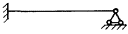
Clamped-supported
|
3.927
|
7.069
|
10.210
|
13.352
|
|
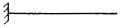
Clamped-free
|
1.875
|
4.694
|
7.855
|
10.996
|
|

Free-free
|
0
|
4.730
|
7.853
|
10.996
|
|
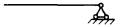
Free-supported
|
0
|
3.927
|
7.069
|
10.210
|
|
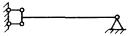
The left one can not
turn, otherwise it is free, the right one is support
|
1.571
|
4.712
|
7.854
|
10.996
|
|
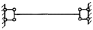
Left and right can not
turn, otherwise they are free
|
3.142
|
6.283
|
9.425
|
12.566
|
|

The left one is
clamped, the right one can not turn, otherwise it is free
|
2.365
|
5.498
|
8.639
|
11.781
|
|
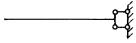
The left one is free,
the right one can not turn, otherwise it is free
|
2.365
|
5.498
|
8.639
|
11.781
|
angles of rotation Х'-
= Х'+
moments (EJX")-
= (EJX")+;
shear forces with due
regard to the reactions of the supports and concentrated mass loads (EJX")-
= (EJX")+ ± R.
Table P8.4
shows the graphs of the first roots of frequency equations for standard rods with
intermediate supports and concentrated masses.
3. CALCULATION OF NATURAL
OSCILLATION FREQUENCY OF ISOTROPIC RECTANGULAR PLATES
3.1. For plates,
supported along the contour, the natural oscillation frequency Ω is determined
by the formula
Table P8.2. Values
of αl of L-shaped rods with clamped ends
|
Scheme
of rod
|
ψ, deg
|
l1/l
= l1/(l1 + l2)
|
|
0
|
0.10
|
0.15
|
0.20
|
0.25
|
0.30
|
0.35
|
0.40
|
0.45
|
0.50
|
|

|
0
|
4.730
|
5.030
|
5.317
|
5.727
|
5.786
|
5.193
|
4.570
|
4.118
|
3.843
|
3.750
|
|
30
|
4.730
|
4.987
|
5.244
|
5.680
|
5.486
|
5.004
|
4.473
|
4.091
|
3.869
|
3.781
|
|
60
|
4.730
|
4.896
|
5.060
|
5.165
|
5.074
|
4.737
|
4.375
|
4.100
|
3.933
|
3.877
|
|
90
|
4.730
|
4.810
|
4.903
|
4.939
|
4.847
|
4.635
|
4.399
|
4.209
|
4.091
|
4.046
|
|
120
|
4.730
|
4.756
|
4.801
|
4.809
|
4.758
|
4.648
|
4.518
|
4.422
|
4.339
|
4.306
|
|
150
|
4.730
|
4.733
|
4.747
|
4.748
|
4732
|
4.702
|
4.662
|
4.626
|
4.600
|
4.591
|
|
180
|
4.730
|
4.730
|
4.730
|
4.730
|
4.730
|
4.730
|
4.730
|
4.730
|
4.730
|
4.730
|
Table P8.3. Values
of αl of L-shaped rods with one-sided clamping (l = l1
+ l2)
|
Scheme
of rod
|
ψ, deg
|
l1/l2
|
|
0
|
2/8
|
4/6
|
5/5
|
6/4
|
8/2
|
∞
|
|
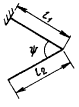
|
0
|
1.875
|
2.053
|
2.623
|
p
|
2.623
|
2.053
|
1.875
|
|
p/3
|
1.875
|
1.946
|
2.226
|
2.362
|
2.316
|
2.005
|
1.875
|
|
p/2
|
1.875
|
1.890
|
2.038
|
2.102
|
2.104
|
1.959
|
1.875
|
|
2p/3
|
1.875
|
1.868
|
1.929
|
1.962
|
1.967
|
1.915
|
1.875
|
|
p
|
1.875
|
1.875
|
1.875
|
1.875
|
1.875
|
1.875
|
1.875
|
Table P8.4.
Values αl of bar systems with intermediate supports and concentrated
masses
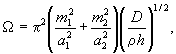
where m1,
m2 = 1, 2, 3, ... is a number of half-waves of the
corresponding forms of natural oscillations; а1, а2
are sizes of the sides; D = Eh3/[12(1 - μ2)]
is a flexural stiffness; h is a plate thickness; ρ is a material
density; μ is a Poisson ratio.
Table P8.5. Values
of α for various boundary conditions
|
Supported-clamped
|
a2/a1
|
0.5
|
0.6
|
0.7
|
0.8
|
0.9
|
1.0
|
|
α
|
6.85
|
5.92
|
5.51
|
5.41
|
5.50
|
5.74
|
|
Supported-free
|
a2/a1
|
0.5
|
0.8
|
1.2
|
2.0
|
3.0
|
5.0
|
|
α
|
4.40
|
2.15
|
1.14
|
0.70
|
0.56
|
0.51
|
|
Clamped-clamped
|
a2/a1
|
0.4
|
0.5
|
0.6
|
0.7
|
0.8
|
0.9
|
|
α
|
9.44
|
7.69
|
7.05
|
7.00
|
7.29
|
7.83
|
|
Clamped-free
|
a2/a1
|
0.8
|
1.0
|
1.3
|
1.6
|
1.9
|
2.2
|
|
α
|
2.70
|
1.70
|
1.41
|
1.33
|
1.36
|
1.45
|
3.2. For plates
supported on two opposite sides x1 = 0; a1,
under different conditions on the sides x2 = 0; a2
natural frequency is determined by the formula
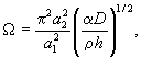
where α is a
dimensionless frequency parameter which values for various boundary conditions
on the sides x2 = 0; a2 are given Table P8.5.
3.3. For plates,
clamped along the contour, the natural oscillation frequency is determined by
the formula
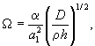
where α is a
dimensionless frequency parameter which values for various ratios of sides a1/a2,
at different half-wave numbers of the corresponding oscillation modes m1
and m2, are given Table P8.6.
4. CALCULATION OF NATURAL
OSCILLATION FREQUENCY OF SHALLOW RECTANGULAR CLADDINGs
4.1. For simply
supported shallow shells with a positive curvature and constant radii of
curvature R1 and R2, the natural
oscillation frequencies are determined by the formula
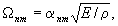
where αnm
is a parameter defined by expression
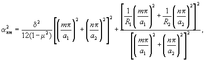
where s is a
shell thickness; m, n is a number of half-waves in directions a1,
a2 for appropriate oscillation modes; a1, a2
are distances between the shell edges along lines with radii of curvature K1
and K2.
Table P8.6.
Values of parameter α for a rectangular plate clamped along the contour
|
m2
|
a1/a2
|
m1
|
|
1
|
2
|
3
|
4
|
5
|
6
|
|
1
|
1
|
35.999
|
73.405
|
131.902
|
210.526
|
309.038
|
428
|
|
1.5
|
27.012
|
65.5
|
126
|
206
|
303
|
422
|
|
2
|
24.58
|
64.1
|
124
|
204
|
302
|
421
|
|
2
|
1
|
73.405
|
108.237
|
165.023
|
242.66
|
340.59
|
458.27
|
|
1.5
|
41.715
|
79.81
|
138.64
|
218
|
316.11
|
436
|
|
2
|
31.833
|
71.08
|
130.35
|
210
|
308.12
|
427
|
|
3
|
1
|
131.902
|
165.023
|
220.06
|
296.35
|
393.36
|
509.9
|
|
1.5
|
66.533
|
103
|
161.234
|
241
|
339
|
457
|
|
2
|
44.779
|
83.2
|
142.38
|
221
|
320.12
|
439
|
|
4
|
1
|
210.526
|
242.66
|
296.35
|
371.38
|
467.29
|
593.8
|
|
1.5
|
100.81
|
136.096
|
193.24
|
271.17
|
369.34
|
488
|
|
2
|
63.34
|
100.80
|
159.49
|
238.35
|
337.08
|
456
|
|
5
|
1
|
309.038
|
340.59
|
393.36
|
467.29
|
562.18
|
676
|
|
1.5
|
144.21
|
178
|
234.65
|
312
|
409
|
529
|
|
2
|
87.26
|
124.2
|
181.79
|
261
|
358
|
478
|
|
6
|
1
|
428
|
458.27
|
509.9
|
583.83
|
676
|
792.5
|
|
1.5
|
195
|
230.04
|
285.4
|
361.90
|
456
|
576.6
|
|
2
|
117
|
151.91
|
209.6
|
287.54
|
382
|
504.3
|
For a
cylindrical shell, it shall be set R1 = ∞; R2
= R; for spherical shell R1 = R2 = R.
5. EXPERIMENTAL METHODS
FOR VIBRATION RESEARCH
5.1. PURPOSE OF EXPERIMENTAL RESEARCHES
5.1.1.
Experimental researches of vibration parameters (vibration deformations and
vibration stresses; displacements, velocities, accelerations and frequency
spectra) of components of structures are carried out in cases when at the stage
of preliminary calculations there is no information about the characteristics
of the actual loads and their spectra.
5.1.2.
Experimental researches of vibrations are carried out with the aim of:
determining the level of
vibrations of equipment for which their maximum permissible values are
specified by technical documentation;
determining the dynamic
characteristics of the components of structures;
determining the
vibration parameters of structures for the subsequent assessment of their
vibration strength;
accumulation of data
necessary to develop and improve methods for calculating and designing
structures with due regard to the effects of vibration loads.
5.2. RESEARCH METHODS
5.2.1. To
determine the parameters of vibration and vibration tension of structures,
methods of vibrometry and dynamic strain measurement are used.
5.2.2. The
research method shall be selected with due regard to the objectives and
conditions of the research.
5.3. OBJECTS OF EXPERIMENTAL RESEARCHES
5.3.1.
Experimental determination of peak, mean, or mean square values of vibration
parameters can be carried out on full-size structures or on their models made
in accordance with the requirements of similarity conditions in hydrodynamics
and dynamic properties of structures.
5.3.2.
Experimental researches on models and full-size structures in solving problems
of items 5.1.1. and 5.1.2 of this Appendix can be carried out at
all stages of the design and development of structures.
5.3.3. When
selecting a research model, one shall be guided by the recommendations of
Sections 5.3 and 5.4 of Appendix 3 hereof.
5.4. EXPERIMENT CONDITIONS
5.4.1. The data on
the operating modes of the structures, equipment characteristics, and coolant
parameters shall be used as the initial information when holding an experiment.
5.4.2. Based on
the initial information on the test object (see item 5.4.1 of this
Appendix), a preliminary analysis of the vibration strength of the structure is
carried out in order to determine areas of increased tension and cross-sections
with maximum vibration displacements.
5.4.3. As
checkpoints of measurements in accordance with item 5.4.2 of this
Appendix, the following is selected:
connection zones of
various structural components;
zones of pipeline
elbows;
(bedding) attaching
points of components of structures;
cross-sections with
possible maximum deflections in case of oscillations in lower forms.
5.5. DYNAMIC STRAIN MEASUREMENT
5.5.1. In
researches of vibration stress of components of structures by the method of
dynamic strain measurement, one shall be guided by the recommendations of items
5.5.1 and 5.5.2 of Appendix 3 hereof.
5.5.2. Universal
recording multichannel light-beam oscillographes and multichannel technical
magnetographs operating in a wide frequency range are used to record fast
processes.
5.6. VIBROMETRY
5.6.1. As the
primary transducers of mechanical vibrations, devices can be used based on such
transformation principles as ohmic, capacitive, inductive, induction, optical,
piezoelectric, etc.
For practical
use transducers and secondary measuring equipment are used, having a lower cut-off
frequency starting with fractions or units of hertz.
5.6.2. To record
the vibration processes, devices specified in item 5.5.2 of this
Appendix are used. Multichannel technical magnetographs can be used as
recording devices necessary for the accumulation and storage of information,
and which make it possible to repeatedly reproduce the required implementations
during analysis of processes.
5.6.3. Spectrum
analyzers are used for frequency analysis with recording the levels of
vibration processes on the corresponding recorders.
5.6.4. Terminology
and definitions of basic concepts in the field of vibration measuring devices
shall comply with GOST 16819-71.
5.6.5. The
selection of vibration measuring devices for experimental researches shall meet
the requirements of GOST 25865-83.
5.6.6. Methods and
means of calibration of vibration measuring devices with piezoelectric
measuring vibration transducers operating in the frequency range of 1-12000 Hz
shall meet the requirements of GOST 8.246-77.
5.6.7. Verification
of vibration measuring devices shall be carried out at least once a year.
5.7. PROCESSING OF THE RESULTS
5.7.1. When
interpreting the oscillographic records and spectrograms, the actual values of
the parameters of vibrations and the main frequencies of the energy spectrum of
vibrations, allowing to establish the nature of the oscillatory process, are
determined.
5.7.2. Processing
of records of vibration processes of a random nature is carried out using the
methods of spectral and correlation analysis.
6. RECOMMENDED METHODS
FOR ASSESSMENT OF VIBRATION STRENGTH OF COMPONENTS OF STRUCTURES
6.1. One of the
criteria for ensuring vibration strength is the condition for detuning the
natural oscillation frequencies of components of structures from discrete frequencies
of deterministic excitation determined in item 1.6 of this Appendix.
The condition
for the detuning of natural frequencies for the first three forms of
oscillations of the components of structures in each plane is written as
Ωi/ω
≥ 1.3 or Ωi/ω ≤ 0.7,
where Ωi
is a lower natural oscillation frequency (i = 1, 2, 3); ω is an
excitation frequency.
For higher
oscillation modes in the presence of high-frequency exciters of vibrations, the
detuning condition is as follows:
Ωi/ω
≥ 1.1 or Ωi/ω ≤ 0.9 (i = 4, 5, ...).
If it is
impossible to fulfill the requirements of these conditions, it is necessary to
show that the vibration levels of the components of structures are within
acceptable limits.
6.2. To
eliminate possible collisions of the single-type components of structures
combined into groups (packages), a condition that satisfies the inequality is
accepted
A < (t – d)/2,
where A is a
maximum amplitude of vibration displacements of a component; t is a
pitch of a component with the largest size d the in cross-section.
For arbitrary
components located with a clearance ∆, this condition is assumed as
|A1|
+ |A2| < ∆,
where A1
and A2 are amplitudes of vibration displacements of the
corresponding components.
For
oscillatory processes of a random nature, the values of amplitudes A, A1,
and A2 are set with due regard to their dispersion with a
given probability; for example, for a normal distribution law with a
probability of 0.997, the values of amplitudes are assumed to be equal to  , where σ is
a standard deviation from the mean value
, where σ is
a standard deviation from the mean value 
6.3. Design
assessment of the durability of components of structures in the case of
imposition of vibration stresses on the main loading cycle is carried out
according to the procedure described in item 5.6 hereof.
When
calculating a2 fracture in the case of a narrowband spectrum,
the maximum mean square amplitude of the high-frequency local stresses and the
corresponding frequency are used.
With a
broadband spectrum, the value of a2 is determined as a sum of
fractures for those amplitudes of local stresses and their corresponding
frequencies that cause fractures of more than 10% of the maximum fracture at
one of the combinations of amplitude-frequency from the entire spectrum. The
cycle asymmetry is determined with due regard to the mean stress assumed to be
equal to the constant local stress from mechanical and thermal loads with the
inclusion of residual tension stresses.
Fracture a*3
is determined with due regard to three maximum amplitudes of high-frequency
stresses without concentration <σa>1, <σa>2,
<σa>3, and corresponding frequencies f1,
f2, f3 for each type of alternating stress
cycle in transients. For low-frequency cycle of the i-th type, by the
formula (5.44) of item 5.6.20 hereof, the values of χ1i;
χ2i, χ3i are determined, and when
determining (a*3) calculated by the formula (5.43)
hereof the coefficient χi is determined by the formula
Share of
fracture a3** is determined by the formula (5.39)
hereof with due regard to the maximum amplitude of the high-frequency stress
during the passage of resonance. The number of cycles is determined with due
regard to the time of operation in a resonance. Asymmetry of the high-frequency
loading cycle is determined by the local stress from mechanical and thermal
loads during operation with due regard to the residual tension stresses for the
middle of the time range corresponding to the resonance.
APPENDIX 9
(recommended)
CALCULATION FOR SEISMIC IMPACTS
1. GENERALIZED RESPONSE
SPECTRA
The
generalized response spectra shown in Fig. P9.1 and
P9.2 correspond to the site seismic intensity of magnitude 9, relative
damping K = 0.02, and are recommended for equipment and pipelines as
part of unified NPPs with VVER-1000. For seismic intensity below magnitude 9,
the acceleration values obtained from Fig. P9.1 and P9.2 are
multiplied by the recalculation coefficient from Table P9.1.
Table P9.1.
Values of recalculation coefficient
Acceleration
values for intermediate marks of equipment or pipelines can be determined by
interpolation.
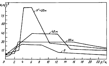
Fig. P9.1.
Generalized response spectra of horizontal oscillations at K = 0.02 and
site seismic intensity of magnitude 9
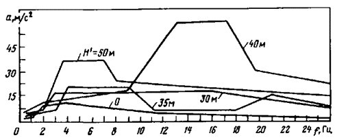
Fig. P9.2.
Generalized response spectra of vertical oscillations at K = 0.02 and
site seismic intensity of magnitude 9
2. UNIFIED METHODS FOR
CALCULATING EQUIPMENT AND PIPELINES FOR STRENGTH FROM SEISMIC IMPACTS
2.1. CONVENTIONAL SYMBOLS, INDICES AND DEFINITIONS
NLC is a nonlinear system
LC is a linear system
DAM is a dynamic analysis method
LCM is a response spectrum method
mii is an
inertia coefficient of the i-th partial system (diagonal element of
matrix [M])
[C] is a
stiffness matrix
[M] is a mass
(inertia) matrix
{x}, { }, {
}, { } are vectors
of relative displacement, velocity, and acceleration, respectively
} are vectors
of relative displacement, velocity, and acceleration, respectively
N is a number of degrees of freedom
[B] is a damping
matrix
{R} is a vector
of reactive forces from "nonlinear connections"
{cos α} is a
vector of directional cosines
 is an acceleration
of the grounds of computational model (accelerogram)
is an acceleration
of the grounds of computational model (accelerogram)
{F} is a
resulting vector of external loads
f is a natural
frequency, Hz
a is an
acceleration, m/s2
H' are elevations of equipment or pipeline,
m
ω is a circular natural
oscillation frequency of equipment or pipeline in air, rad/s
 is a circular
natural oscillation frequency of equipment or pipeline in liquid, rad/s
is a circular
natural oscillation frequency of equipment or pipeline in liquid, rad/s
C is a stiffness coefficient, N/m
C0 is a shift coefficient
M is a weight of a part of equipment or pipeline
 is an added mass
of fluid, kg
is an added mass
of fluid, kg
 is a reduced mass
of a part of equipment or pipeline, with due regard to the added mass of fluid,
kg
is a reduced mass
of a part of equipment or pipeline, with due regard to the added mass of fluid,
kg
M1 is a mass per unit length of equipment
or pipeline, kg/m
M0 is a mass of fluid displaced by a part
of equipment or pipeline immersed in it, kg
g – 9.81 m/s2
– free fall acceleration
G is weight, N
q is force, N
m is a moment
of force, N · m
E is a modulus of elasticity, N/m2
μ is a Poisson ratio
x is an added
mass coefficient
M' is a function of coordinates of a part
of equipment, representing the distribution of its mass, kg
A is a function of coordinates of a part of
equipment that determines the shape of the oscillation considered and
represents the ratio of the displacements of the points of the part of
equipment to the displacements of the reference point, which is assumed to be
equal to one
δ is displacements, m
As is a cross-sectional
area, m2
l is a lenght
of the component of structure, m
d is a
diameter, m
t is a pitch
of holes, m
s is a
thickness, m
J is a moment of inertia of the cross-section, m4
J0 is a moment of inertia of mass rotation,
kg · m2
i is an
inertia radius, m
z is a number
of the components of structures
 is a cylindrical
stiffness, N · m
is a cylindrical
stiffness, N · m
Indices
i – for
parameters related to the i-th part of equipment
st – for
parameters related to static load (for the own weight)
kr – for
critical value when calculating stability
red – for
parameters related to the reference point
l – for
parameters related to legs
w – for
parameters related to bolts
a – outer
DEFINITIONS
Supporting connection (support)
is a structure that connects equipment or pipeline with an anchorage point
(anchor bolt, mounting leg, supporting flange, shock absorber, etc.).
Non-supporting connection is a
structure that connects equipment units together (branch pipe, bellows,
pipelines, etc.).
A shock absorber is a mechanism or a
hydraulic mechanism that connects equipment to its anchorage point in order to
increase the strength of this equipment under seismic loads. The design of the
shock absorber shall ensure its low stiffness during temperature displacements
of equipment and greater stiffness under seismic loads.
The fluid in which the
oscillating body is located is considered infinite if the size of the
vessel in the direction of the body oscillation is more than 5 times greater
than the maximum size of body in this direction.
2.2. CALCULATION
METHOD SELECTION
The
calculation method is selected in accordance with Table P9.2. Pipelines
are allowed to be considered as linear systems.
Input data on
seismic impact are accelerograms or response spectra.
Table P9.2. Recommendations
for selection of the calculation method and input data of seismic impact
|
Type
of calculation model
|
Calculation
method
|
Impact
input data
|
|
LC
|
DAM or LCM
|
Accelerograms or
response spectra
|
|
NLC
|
DAM
|
Accelerograms
|
2.3. PRINCIPLES OF MAKING A MECHANICAL MODEL AND
CALCULATION OF ITS PARAMETERS
2.3.1. Principles
of making and requirements to the mechanical model of equipment.
To carry out
calculations of equipment components for strength from seismic impacts, a
mechanical model of equipment consisting of masses linked together and with
anchorage points by connections is made. Equipment components with low weight
(mount fitting, shock absorber, etc.) are introduced into the model only as a
connection with a certain stiffness. If the equipment consists of separate
units, rigidly fixed and having non-supporting connections, these links are not
considered in further calculations.
The design
mechanical model of equipment or pipelines shall reflect the basic dynamic
properties of the considered structure, satisfy the volume of the required
design verification and the capabilities of computer calculation programs and
(or) selected calculation methods.
2.3.2. Calculation
of the basic parameters of the mechanical model of equipment.
2.3.2.1. For a part
of equipment that can be schematized as a concentrated mass with a connection,
the mass and stiffness coefficient are determined on the basis of the drawings.
To calculate the stiffness coefficient, the methods of resistance of materials
are used.
The circular
natural frequency is determined by the formula

2.3.2.2. To
determine the mass, stiffness coefficient, and circular natural frequency of
parts and assembly units with distributed parameters, the reduction method is
used as follows:
1) a certain
deflection curve is set, which can occur during oscillations (at first
approximation it is a static deflection curve from weight loads);
2) a reference
point is selected (the point can be selected arbitrarily, but the following
condition shall be met: when oscillations of the structure, the reference point
displacement is different from zero);
3) a reduced
mass Mred is calculated for the given reference point;
4) a circular
natural frequency is determined by the formula
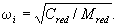
In general,
for part of the equipment with distributed parameters
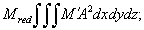

where  is a
potential energy of a part of equipment when displacement of a reference point
is equal to one. Values of Mred and Cred
can also be calculated by the formulas
is a
potential energy of a part of equipment when displacement of a reference point
is equal to one. Values of Mred and Cred
can also be calculated by the formulas
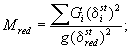
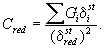
Reduced
stiffness coefficients can be determined by the methods of resistance of materials.
And for parts of small length (s/l ≥ 0.3), the effect of shear
shall be considered by multiplying the reduced stiffness coefficient by the
shear coefficient CQ, determined depending on the shape of a
part.
2.3.2.3. If, for a
part of equipment with a constant cross-section (constant mass per unit length M1),
the static deflection curve from concentrated force F applied in the
reference point is selected as the deflection curve, then
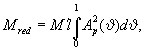
where  is a
relative static deflection curve from force F;
is a
relative static deflection curve from force F;  is a
relative coordinate.
is a
relative coordinate.
In this case,
the reduced stiffness coefficient is equal to the force (or moment) causing the
displacement of the reference point equal to one in the direction of the
action.
2.3.2.4. The reduced
mass of the part of equipment in a liquid medium is determined with due regard
to the added mass of fluid by the formula
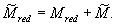
The added mass
of fluid is calculated by the formula

2.3.2.5. For parts
of equipment that are in infinite fluid, x shall be assumed in accordance with
Table P9.3.
2.3.2.6. The
coefficient x for cylindrical components that are in limited volumes of water
can be determined by Fig. P9.5.
2.3.2.7. The mass
per unit length of the rod , with due regard to the
added mass, is calculated by the formula
, with due regard to the
added mass, is calculated by the formula

where M2
is an added mass per unit length of fluid determined by the formula M2
= xM01, M01 is a mass of fluid displaced by
a rod of unit length.
2.3.2.8. For a
vessel or rod completely filled with fluid, as well as for vertical cylindrical
vessels with a ratio of the fluid height to the vessel’s radius greater than
four, the added mass of fluid is equal to the mass of fluid.
Table P9.3. Value
of coefficient x
|
Form
of equipment part
|
Direction
of displacement when oscillations
|
x
|
|
Long cylinder (l
≥ 8d)
|
Perpendicular to the
longitudinal axis
|
1.0
|
|
Short cylinder (l
< 8d)
|
Same
|
According to Fig. P9.3
|
|
Pack of cylindrical
rods
|
"
|
According to Fig. P9.4
|
|
Ball
|
Any
|
0.5
|

Fig. P9.3. Added
mass coefficient for single cylindrical rods with oscillations in an infinite
volume of fluid
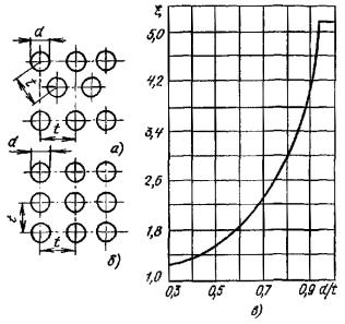
Fig. P9.4. Added
mass coefficient for packs of rods:
a is a
location of the rods on a triangular grid; b is a location of the rods
on a square grid; c is coefficient x
2.3.2.9. The
circular natural frequency of the part of equipment immersed in fluid is
determined by the formula

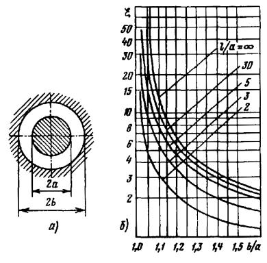
Fig. P9.5.
Scheme (a) and dependence of the added mass coefficient on b/a
for single rods with oscillations in a limited volume of fluid (b). At l/a
< 2 in all cases, it shall be assumed x = 1.0
or
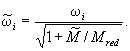
2.3.2.10. The free
oscillation frequency of the part of equipment, which can be schematized in the
form of a rectilinear single-span beam of constant cross-section, is determined
by the formula

where x is a
coefficient determined in accordance with Table P9.4.
For the same
parts of equipment, Table P9.4 gives the values of the reduced
stiffnesses and the reduced masses.
2.4. CALCULATION OF STANDARD STRUCTURES, ASSEMBLY
UNITS AND ITEMS OF EQUIPMENT
2.4.1. Selection
of design models.
2.4.1.1. The design
models of the main standard parts of equipment are shown in Fig. P9.6
and P9.7.
2.4.1.2. When
calculated in the horizontal direction, the pull-out part of the reactor
consisting, for example, of the removable screen connected to the plate in its
lower part is considered as a cantilever cylindrical beam, which is loaded with
a uniformly distributed screen mass and a concentrated plate mass. The upper
contour of the beam is rigidly clamped, and the lower contour is supported by a
rigid slab.
Table P9.4. Values
of reduced stiffnesses and masses
|
Design
diagram
|
x
|
Cred
|
Mred
|
|
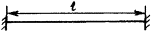
|
22.4
|

|
0.4M1l
|
|
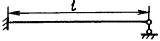
|
15.4
|

|
0.43M1l
|
|

|
9.86
|

|
0.5M1l
|
|
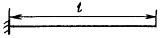
|
3.52
|

|
0.25M1l
|
2.4.1.3. The process
channel is considered as a rod of variable cross-section having a rigid
restraint in the base plate and intermediate hinge supports in the places where
channel passes through spacer perforated plates. The rod is loaded with
distributed mass.
2.4.1.4. The drive
of the Control and Protection System (CPS) is considered as a cantilever bar
system consisting of tubular rods of a step-variable cross-section, which are
loaded with distributed natural mass and concentrated mass of drive mechanisms.
The bar system has a pliable restraint in the lid due to the flexibility of the
CPS drive mounting unit to the lid.
2.4.1.5. Tubes of
heat exchangers are considered beams of constant cross-section, clamped in
supports (tube plates, diaphragms) and loaded with a uniformly distributed
mass.
2.4.1.6. Plates,
diaphragms, tube plates, lids, flat screens and other similar structures are
considered as solid plates. Depending on the mounting design, the contour of
the plate is considered to be clamped or simply supported. In case of the
calculation of tube plates or other perforated structures, the above
characteristics are introduced into the calculation, which reduce the
perforated plate hardness to solid.
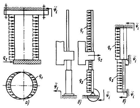
Fig. P9.6.
Design models for standard units:
a is a
pull-out part; b is a CPS drive; c is a process channel
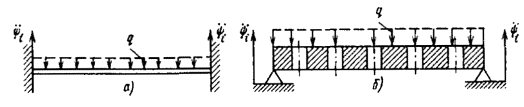
Fig. P9.7.
Design models for standard units:
a is a heat
exchanger tube; b is a perforated plate
It is assumed
that the plate is loaded with a uniformly distributed mass.
2.4.2. Calculation
of the basic parameters of the mechanical model for standard parts.
2.4.2.1. When
calculating the natural oscillation frequency of package units, the weight of
mount fittings is not taken into account due to its smallness compared to the
weight of equipment.
The reduced
stiffness of the mount fitting is determined by the formula
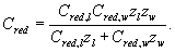
For the bolt
in the direction of its axis
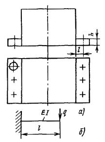
Fig. P9.8. Structure
sketch (a) and the design model (b) of the mount fitting with
beam type legs
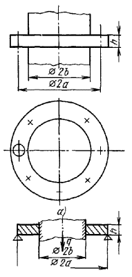
Fig. P9.9. Structure
sketch (a) and the design model (b) of the mount fitting with
supporting flanges
The reduced
stiffness coefficients of the legs (supporting flanges, pressure flanges) are
calculated:
for beam type leg (Fig. P9.8)
– by the formula

for supporting flange
(Fig. P9.9) – by the formula
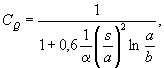
where a, b
are sizes of the supporting flange.
Table P9.5. Value
of coefficient α
|
a/b
|
1.05
|
1.1
|
1.15
|
1.2
|
1.25
|
1.5
|
2.0
|
3.0
|
4.0
|
5.0
|
|
α
|
0.0001
|
0.0004
|
0.0014
|
0.003
|
0.005
|
0.025
|
0.088
|
0.209
|
0.293
|
0.35
|
Numerical
values of the coefficients a are given in Table P9.5.
For sectoral
legs (Fig. P9.10)
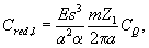
where m is a
length of the arc of one leg, measured around a circle by radius a. The
value of CQ is determined in the same way as for the
supporting flange.
For legs and
supporting flanges, supported by stiffeners (Fig. P9.11),
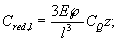
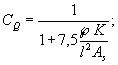
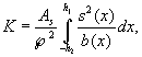
where z is a
number of sections; h1, h2 are distances,
respectively, from the upper and lower edges of the cross-section; s(x)
is a static moment of inertia of the cross-sectional area; b(x)
is a width of a section.
For fastening
with boots (Fig. P9.12)
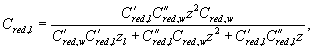
where C'red,l
is a reduced stiffness coefficient of boots, calculated by the formulas for
beam type legs; C"red,l is a reduced
stiffness coefficient of supporting flange calculated by the formulas for
supporting flanges; z is a number of boots;
C'red,w = Cred,w(aw/bw)2;
aw, bw
are sizes of boots (see Fig. P9.12). For pressure flange (Fig. P9.13)
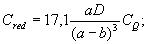
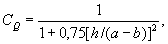
where a, b,
h are sizes of pressure flange (see Fig. P9.13).
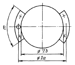
Fig. P9.10.
Scheme of the mount fitting with sectoral legs
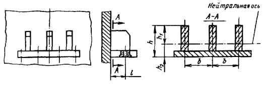
Fig. P9.11.
Scheme of enforcement of legs and supporting flanges by stiffeners
|
нейтральная
ось
|
neutral axis
|
2.4.2.2. The reduced
stiffness coefficients and the mass of the cylindrical body of equipment with
attachment to the foundation according to the schemes shown in Fig. P9.14,
a and b are determined in the following order.
When calculating
oscillations in the direction of the body axis in accordance with the scheme
shown in Fig. P9.14, c,
Cred = (EAs)/l;
Mred = 0.33M1l.
For bodies
with fastening in the middle part (Fig. P9.14,b)
l = l1
+ l2.
When
calculating oscillations in the transverse direction (Fig. P9.14,d)
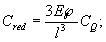
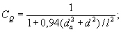
Mred = 0.26M1l.
For
double-seat body (Fig. P9.15) with oscillations in a direction
perpendicular to the axis
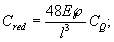
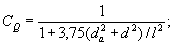
Mred = 0.5M1l.
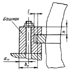
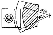
Fig. P9.12.
Scheme of the mount fitting with boots
2.4.2.3. The reduced
stiffness coefficient and mass for a cantilevered screen are determined in the
same way as for the bodies shown in Fig. P9.14. For screens with limit
stops (Fig. P9.16) when calculating oscillations in the transverse direction
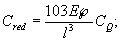
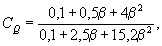
where

Mred = 0.43M1l.
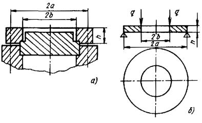
Fig. P9.13. Structure
sketch (a) and the design model (b) of the mount fitting with
pressure flanges
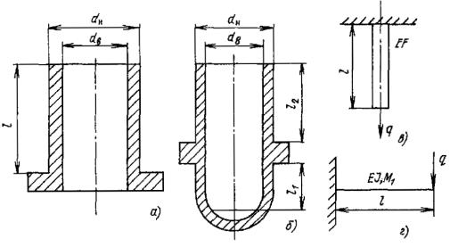
Fig. P9.14. Scheme
of fastening the body to the foundation in the lower (a) and middle (b)
parts and the design model for the longitudinal (c) and transverse (d)
oscillations
Design values
of Cred and Mred in case of oscillations in
the direction of the screen axis are determined in the same way as for bodies
in case of oscillations in the longitudinal direction (see Fig. P9.14, c).
2.4.2.4. When
calculating the reduced coefficients of stiffness and weight of a lid or
perforated plate at h/a > 0.3 (Fig. P9.17), the lid or
plate is considered as a concentrated mass. At h/a ≤ 0.3 in case
of transverse oscillations, the values of Cred and Mred
are found from the following dependencies:
for lids, plugs and
other components such as solid round plates
Cred =32.4D/a2;
Mred = 0.3M;
for perforated plates
Cred =32.4Dφb/a2;
Mred = 0.3M,
where φb is
an attenuation coefficient when bending.
2.5. LINEAR SPECTRAL CALCULATION METHOD
2.5.1. The linear
spectral method is based on the reduction method, which makes it possible to
reduce a linear system with N degrees of freedom to N equivalent
systems with one degree of freedom, the imposition of oscillations of which
gives the total oscillation of the original system.
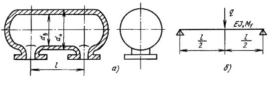
Fig. P9.15. Structure
sketch (a) and the design model (b) of fastening of the
double-seat body to the foundation
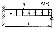
Fig. P9.16.
Scheme of screen with limit stop
2.5.2. To use the
reduction method, the eigenvalues and eigenvectors of a system of homogeneous
algebraic equations of the following form are determined
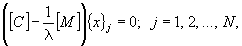
where {x}j
= {x1j...xij...xNj}
is the j-th eigenvector corresponding to eigenvalue λj.
Provided that,
the natural frequency of the j-th oscillation mode

2.5.3. When
determining seismic loads, the calculation considers S of lower
oscillation modes (S ≤ N), the natural frequency of which does
not exceed the highest frequency for which response spectra are given.
2.5.4. The seismic
load acting in the direction of the i-th generalized coordinate and
corresponding to the j-th form of natural oscillations of the system is
determined by the formula
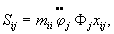
where  is an
acceleration determined by the response spectrum for the frequency ωj;
is an
acceleration determined by the response spectrum for the frequency ωj;

Fig. P9.17. Structure
sketch (a) and the design model (b) of lids and perforated plates
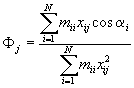
is a constant of the j-th
form of oscillations; αi is an angle between the directions
of the seismic impact and the i-th generalized coordinate.
2.5.5. The internal
forces (stresses) in the connections of the calculation model are determined
from the effect of the seismic loads Sij statically applied
to the assemblies separately and summed for each mode of oscillations by the
formula
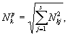
where Nkp
is a design force in the k-th considered cross-section; Nkj
is a force of a certain type in the cross-section k for j-th mode
of oscillations.
2.5.6. The
relative displacements of the calculation model in the direction of the i-th
generalized coordinate of the j-th mode of oscillations are determined
by the formula
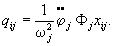
The design
value of the displacement in the direction of the i-th generalized
coordinate is found as follows:

This
dependence can be used to determine velocities and accelerations if the
following condition is met simultaneously
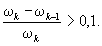
If this
condition is not met, then the design value is determined by the formula
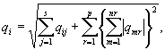
where p is a
number of natural frequency groups for which the condition is met (ωk
– ωk-1)/ωk < 0.1.
2.5.7. The
resulting values of internal forces, stresses, as well as displacements,
velocities and accelerations in the structure, which was represented by a set of
flat rod design models and calculated separately for each of the mutually
perpendicular directions, are determined by the formula

where Pkp
is the resulting value of the parameter in the k-th cross-section
(assembly) considered; Pkn is a value of a parameter of a
certain type in the k-th cross-section (assembly) obtained for the n-th
direction of displacements.
In this case,
the conditions specified in item 2.5.6 shall be taken into account.
This method of
summation can also be applied when using other methods of calculation.
2.6. METHOD OF DYNAMIC ANALYSIS OF SEISMIC
RESISTANCE
2.6.1. When
performing calculations by the method of dynamic analysis, accelerograms of
movement of the bases (supports) of the calculation model are set as external
seismic impact.
2.6.2. Dynamic
analysis of systems with a finite number of degrees of freedom, inter alia
non-linear ones with the same regularity of the kinematic excitation of
supports, is carried out by the methods of numerical integration of systems of
differential equations of the form of
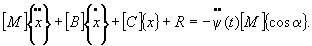
2.6.3. The vector
of reactive forces {R} acting in the direction of the generalized
coordinates of the system is the sum of the reactions of additional non-linear
connections of the system: dampers, shock absorbers, elastic stops with
clearances (including connections), components of dry friction, etc.
2.6.4. The
resulting vector of external loads acting on the system at any moment of time
is determined by the formula
{F} =
[C]{x}.
2.6.5. Based on
the calculated value of the vector {F}, internal forces and stresses are
determined in the design cross-sections of the system.
3. PROCEDURES FOR
CALCULATING PIPELINES FOR SEISMIC IMPACTS
3.1. INTRODUCTION
The procedures
given in this Section can be used to calculate pipelines of the category II.
The procedures
are based on the statistical theory of seismic resistance of structures.
3.2. PROCEDURE OF CALCULATION OF PIPELINES BY
RESPONSE SPECTRUM
3.2.1. Additional
conventional symbols
x, y, z
are pipeline coordinate system indices
(σs)s2
is a group of reduced membrane and general bending stresses only from seismic
impacts (response spectrum of OBE*)
* OBE is an
operating basis earthquake.
(σs)s2,x;
(σs)s2,y; (σs)s2,z
are stress components (σs)s2
σmax,x(y,z)
is a maximum reduced stress in the pipeline from the loads of proper weight
applied along the axes x, y and z
f1,x(y,z) is the first
natural oscillation frequency about the axis x (y or z)
Kh is a coefficient of
change of maximum acceleration (seismic impact) according to the height of
structure. For NPP with VVER, the values of this coefficient are given in Table
P9.6
A0max,x(y,z) is a
coefficient equal to the maximum acceleration value in fractions of g in
the OBE response spectrum for the zero elevation in the direction of seismic
impact x (y, z)
Ahmax,x(y,z) – the same
for the maximum elevation of fixing of the fixed support of pipeline
Ahf1,x(y,z) is a
coefficient equal to the value of acceleration in fractions g for the
corresponding first natural frequency in the OBE response spectrum, with the
direction of seismic impact x (y, z), with due regard to
the maximum elevation of fixing of the fixed support of pipeline
Δsj,x(у,z)
is a displacement the center of gravity of the i-th section of the
pipeline from seismic effects along the axis x (y, zg)
δjx(y,z)
– the same from the proper weight loads along the axis x (y, z)
Table P9.6. Coefficient
Kh for NPP with VVER
|
Construction
characteristic
|
Maximum elevation of fixing
of pipeline
|
|
10 m
|
20 m
|
30 m
|
40 m
|
|
Horizontal components
|
Vertical component
|
Horizontal components
|
Vertical component
|
Horizontal components
|
Vertical component
|
Horizontal components
|
Vertical component
|
|
Box (massive reinforced concrete
structure)
|
1.2
|
1.0
|
1.5
|
1.2
|
1.75
|
1.6
|
2.0
|
2.0
|
|
Containment
|
1.2
|
1.0
|
1.6
|
1.2
|
2.0
|
1.6
|
2.5
|
2.0
|
|
Space framework (frame arrangement of
bearing components)
|
1.4
|
1.4
|
1.8
|
1.8
|
2.25
|
2.2
|
3.0
|
3.0
|
Note. The
table is applicable for soils having a modulus of elasticity of E ≥ 104
MPa. At Е < 105 MPa, the values of coefficient Kh
from this Table shall be multiplied by 1.5.
3.2.2. General
3.2.2.1. The
pipelines are calculated for seismic impacts after performing calculations for
static and cyclic loads and confirming their strength under these loads.
3.2.2.2. This method
of calculation involves the static calculation of stresses (σs)s2
in the pipeline components.
The
calculation is carried out using programs and results of strength static
calculations of pipelines. At the same time, the calculation when designing
mass loads on the coordinate axes x, y, z is added to the
usual static calculations.
For programs
where it is provided to set the load from the proper weight only in one
(vertical) direction, it is necessary to change the directions of the axes of
coordinates so that the load of the proper weight can be set in the horizontal
direction.
3.2.2.3. The
calculation of σmax,x(y,z) is carried out at a
temperature of 20 °C, zero values of the "inherent" displacements of
the terminal clamped cross-sections, and an internal pressure equal to zero.
3.2.2.4.
Calculation: is carried out for the modulus of elasticity of the material
corresponding to the design temperature of the pipeline wall.
3.2.2.5. Strength
calculations, as well as selection of additional supports necessary to ensure
strength under seismic impacts, are carried out separately for each direction
of seismic impact;
To assess the
strength of the joint action of a three-component seismic impact, stresses from
seismic loads are determined as the square root of the sum of squares of
stresses from seismic loads obtained for individual directions of seismic
impact.
When automated
calculations, the total reduced stresses from the considered static and seismic
loads are determined by the forces obtained from the combined action of these
loads.
3.2.2.6. Seismic
impact is given by the OBE response spectra.
3.2.2.7.
Recommendations for selection of design models for the pipeline system are as
follows:
when considering
separately the oscillations of pipelines with respect to any of the three
coordinate axes (x, y, z), only those supports which limit
the displacements of pipelines along this axis are considered;
the design model of the
pipeline system is made up with due regard to all branches and connected
equipment; the influence of branches not included in the design model shall be
considered in the form of added masses and corresponding connections.
3.2.3. Criterion
of seismic strength.
Criterion of
seismic strength is determined with due regard to the requirements of Table 5.14
hereof. The values of this criterion are determined by the dependence
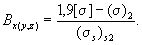
Pipeline
strength conditions
Bx(y,z) ≥ 1. (P9.1)
3.2.4. The
following input data are necessary for the calculations:
1) geometrical
and operational parameters of the pipeline system;
2) stiffness
properties of the supports;
3) values of
stress (σ)2 according to the results of static strength calculations
of pipelines for normal operation;
4) OBE
response spectra at the zero elevation and at the elevations of fixing of the
fixed pipeline supports.
3.2.5. The
sequence of the calculation.
The
calculation is carried out in the following sequence:
1) (σs)s2
is determined for the directions of OBE seismic impacts coinciding with the
direction of action of proper weight loads projected on the coordinate axes of
the pipeline system;
2) the strength of the pipeline by the
seismic strength criterion is assessed (P9.1);
3) the strength of supporting structures
is checked with due regard to the loads from seismic impacts;
4) a positive
conclusion about the strength is given provided that the strength requirements
of items 3.2.5.2 and 3.2.5.3 are met.
3.2.6. Calculation
of (σs)s2.
Calculation of
stresses from seismic loads is carried out according to the following
dependencies:
1) in the
absence of a response spectrum at the elevation if fixing of fixed supports
(σs)s2,x
= 1.3A0max,xKhσmas,x
(P9.2)
and also for other
directions of seismic impact;
2) in the
presence of a response spectrum for the elevation if fixing of fixed supports
(σs)s2,x
= 1.3Ahmax,xKhσmas,x
(P9.3)
and also for other
directions of seismic impact. When the seismic strength condition (P9.1)
is met, the strength is ensured and further calculations can be omitted;
3) if the
strength condition (P9.1) is not met, the calculation is carried out
with due regard to the first natural oscillation frequency
(σs)s2,x
= 1.3Ahf1,xσmas,x
(P9.4)
and also for other
directions of seismic impact.
The first
natural oscillation frequency for a particular direction of seismic impact is
allowed to be determined using displacement values obtained as a result of
calculations when a pipeline has a load of proper weight projected on
coordinate axes x (y or z):
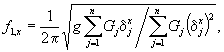 (P9.5)
where Gj
is a weight of the j-th segment of the pipeline from the span between
the corresponding points of the scheme used for static calculations; δjx
(δjy, δjz) are
displacements of the center of gravity of the j-th segment when the
pipeline has a load of proper weight projected on one of the directions of the
axes of coordinates by the formula (for example, along axis x)
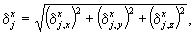 (P9.6)
where δxj,x,
δxj,y, δxj,z
are projections of the displacements of the j-th cross-section on axis x
from the proper weight loads applied along axis x.
For other
directions of seismic impact, the frequency is calculated similarly.
For cases when
all the branches included in the design model differ significantly in stiffness
and inertial characteristics, the frequencies f1,x, f1,y,
f1,z are calculated for each branch according to the
displacements created by proper weight loads, taking into account the joint
operation of all the branches.
For pipelines
containing branches, which the type parameter  differs by
no more than 2 times from the corresponding parameter of the main pipeline, the
seismic strength assessment is carried out according to the first natural
frequency (fx, fy, fz).
differs by
no more than 2 times from the corresponding parameter of the main pipeline, the
seismic strength assessment is carried out according to the first natural
frequency (fx, fy, fz).
To calculate
the indicated frequencies, other methods can be used, which are in good
agreement with the capabilities of the static calculation program.
If the strength
conditions are not met, then additional supports or shock absorbers are
installed in the direction of those coordinate axes for which the strength
conditions are not met. Then, according to the scheme with additional supports
and shock absorbers, the static calculation of the pipeline for
self-compensation is repeated and the calculations for seismic impacts are
repeated according to item 3.2.5 of this Section.
3.2.7.
Determination of seismic loads from the pipeline on the equipment and fixed
supports.
The
equivalence coefficients of seismic loads are determined statically by the
formulas


 (P9.7)
For fixed
supports and equipment, the seismic load is determined as the product of static
loads from the normal operation modes and coefficients Kx, Ky,
Kz:
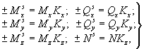 (P9.8)
where M, Q,
and N are moment, transverse and longitudinal force.
It is assumed
that seismic loads coincide in sign with static loads from normal operation
modes.
3.2.8.
Determination of seismic loads for intermediate supports.
The value of
the seismic load on the intermediate sliding supports or simple suspensions is
determined by the dependence
±Ns = NjKz,
(P9.9)
where Nj
is a load on this support according to the results of static calculations from
the normal operation modes.
To determine
additional loads on the spring supports, a coefficient K0s
is introduced:
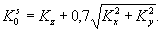 (P9.10)
For this case,
seismic loads are equal to the forces affecting supports from static loads of
normal operation modes, multiplied by the coefficient K0s,
that is
±Njs = K0sNj.
(P9.11)
3.2.9. Appointment
of seismic protection arrangements. Procedures for the appointment of seismic
protection arrangements are carried out if the seismic strength is not provided
and are as follows:
1) the type of
additional supports is selected: fixed supports (then the scheme is divided
into several independent ones), intermediate sliding supports, simple or spring
suspensions, shock absorbers;
2) the
installation location of supports or shock absorbers, their preliminary number
are determined, and in accordance with item 3.2.3. seismic strength
criterion Bx(y,z) are found.
Assuming the
entire pipeline length as L, it is considered that, at Bx
= 1, the length of the pipeline projection onto the x axis, equal to Lx,
satisfies the seismic strength condition.
When Bx
< 1, the seismic strength condition is not met, respectively, the length Lx
may contain two or more sections, and the number of additional supports or
shock absorbers on the length Lx is greater than or equal to
one. The length of the section satisfying the seismic strength condition,
Lx = BxLx.
(P9.12)
Then the
required number of additional supports or shock absorbers n = Lx/lx
(the number of supports is rounded upwards to the whole number). This is the
minimum number of supports at which the seismic strength condition may be
satisfied.
Installation
locations of the supports are determined constructively, and the length of the
inter-support sections shall not be less than lx;
3) the static
calculation of σmas for the coordinate axis, relative to which
additional supports or shock absorbers are installed, is carried out;
4) the seismic
strength condition is checked in accordance with item 3.2.5.
The final
number of shock absorbers is determined after the checking calculation.
It is
advisable to unify the power of shock absorbers according to the value of
maximum effort.
3.2.10. In cases
when it is required to carry out seismic resistance assessment by
displacements, for calculating displacements from seismic loads it is allowed
to use the formula
δsj,x = 1.3Ahf1,x(y,z)δjx(y,z). (P9.13)
If there are
no floor-by-floor response spectra, displacement calculations can be performed
using the formulas
δsj,x = 1.3A0f1,x(y,z)Khδjx(y,z). (P9.14)
or
δsj,x = 1.3A0max,x(y,z)Khδjx(y,z). (P9.15)
The total
displacements from seismic loads in each j-th cross-section of the
pipeline can be calculated from the dependence
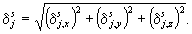 (P9.16)
3.3. PROCEDURE OF CALCULATION OF PIPELINES BY
GENERALIZED SEISMIC LOAD
3.3.1. Three
separate calculations of the pipeline are carried out for the effect of the
weight load (calculations 1, 2, 3). The load is applied in stages in a vertical
direction (along the z axis) and in two horizontal directions (along the
x and y axes). In each individual calculation, the reduced
stresses (σ)x, (σ)y, (σ)z,
forces in the supports and components of the displacement of the cross section
of the pipeline in the direction of the main axes (x, y, z)
are determined. The pressure in the pipeline and the tightening force of the
elastic supports are assumed equal to zero. When calculating, the stiffness of
all supports and shock absorbers is considered.
3.3.2. The
approximate value of the first natural oscillation frequency of the pipeline is
determined by the formula
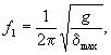
where δmax is
a maximum absolute value of the components of displacements of the pipeline
along one of the axes under the action of weight load separately for each of
the accepted directions.
3.3.3. The
resulting value of the spectral acceleration is determined by the formula
where Ax(f1),
Ay(f1), Az(f1)
are accelerations (in fractions g) determined by the OBE response
spectrum at a frequency f1, set for three directions of
seismic impact at the highest elevation of pipeline fixing.
3.3.4. Values of
the reduced stresses in the cross-sections of the pipeline from the action of
seismic and operational loads are determined by the formula

where (σ)x,
(σ)y, (σ)z are reduced stresses obtained by
calculations 1, 2, 3.
For
rectilinear pipeline segments, it is allowed to determine the stress (σs)
as follows:
if  then
then
(σs)2
= σθ;
if  then
then
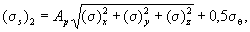
where σθ is a
circular general membrane stress in the pipe from the design pressure.
3.3.5. Efforts of
pipeline impact on equipment under the joint action of operational and seismic
loads are determined by the formula
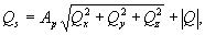
where Qs
is a force vector component (any of the forces along the axes x, y,
z, any moment regarding axes x, y, z) with joint
action of loads; Q is a value of the same component, determined by the
calculation of the pipeline to the effect of operational loads only; Qx,
Qy, Qz are values of the same component
determined in calculations 1, 2, 3.
3.3.6. The loads Psz
(along the z axis) of elastic (spring) suspensions under the joint
action of seismic and operational loads are found by the formula
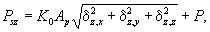
where δzx,
δzy, δzz are displacements along the z-axis
of the pipeline at the place of installation of the suspension, determined in
the calculations 1, 2, 3; P is a suspension load along the z axis
under normal operations; K0 is a suspension stiffness
coefficient.
3.3.7. Reactions
of the sliding supports and the guide supports are calculated similarly to item
3.2.5. For example, the reaction along the z axis is determined
by the formula
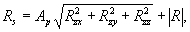
where Rzx,
Rzy, Rzz is a support reactions along the z
axis determined in the calculations 1, 2, 3; R is a support reaction
along the z axis, determined by the calculation of pipelines for
operating loads only.
3.3.8. Reaction of
the shock absorber is determined by item 3.3.7, and its response under
operating loads is assumed to be zero.
3.3.9. The seismic
strength assessment according to the obtained reduced stresses (σs)2
is carried out in accordance with Section 5.11 hereof.
APPENDIX 10
(recommended)
SELECTION OF BASIC SIZES OF FLANGES,
PRESSURE RINGS, AND FASTENERS
1. CONVENTIONAL SYMBOLS
D is an inner diameter of flange, mm
Dw is a diameter of
circumference of pins, mm
Df is an outer diameter of
flange and clamp of slip-on flange, mm
Dm is a design diameter of
gasket, mm
Dm1, Dm2
are mean diameters of shaped gaskets, mm
Dd is an outer diameter of
gasket, mm
D1 is an inner diameter of pressure ring,
mm
D2 is an outer diameter of pressure ring,
mm
d0 is a hole
diameter for pins, mm
d1 is an inner
diameter of pin thread, mm
ds is a minimum
pin rod diameter, mm
dc is a
diameter of the central hole in pin, mm
h1 is a height
of the cylindrical part of the disc flange of thickness, s1,
mm
h2 is a height
of the tapered part of the disc flange, mm
hf is a height
of flange and supporting clamp, mm
hf1 is a height
of the pressure ring, mm
s1 is a nominal
wall thickness of the cylindrical part of the flange, mm
s2 is a nominal
wall thickness of the conical adapter at the base, mm
lw is a pin
pitch, mm
b0 is a gasket
width, mm
b is an
effective width of gasket, mm
δ is a gasket thickness,
mm
q0 is a
specific pressure on the gasket when tightening pins, MPa
p is a design
pressure, MPa
ph is a
hydrotest pressure, MPa
Fd is a gasket clamping
force, N
F2h is a force providing
tightness at hydrotest, N
Fp is a tension force in
the pins from the design pressure, N
Fph is a tension force in
the pins from the hydrotest pressure, N
F0 is a pin tightening force, N
F1 is a force in the cylindrical section of
a flange from the action of inner pressure, N
F2 is a force providing tightness at the
operating pressure, N
F3 is a force from the pressure of the
medium on the inner section of a flange face, N
[σ] is a permissible
nominal stress in a flange, MPa
[σ]w
is a permissible nominal stress in pins, MPa
M is a maximum bending moment, N · mm
ei are arms of
force action, mm
z is a number
of pins
2. SELECTION OF SEALING
2.1. To ensure
the tightness of the equipment, it is recommended to select the sealing
depending on the type and design of the flange connection according to Fig. P10.1
and Table P10.1.
To select the
gasket material use the recommendations given in Table P10.2.
2.2. The outer
diameter of the gasket is determined by the formula
Dd = D +
2b0 + 2u, (P10.1)
where u is a
distance from the inner edge of the flange to the inner diameter of the gasket;
depending on the type, material of the gasket and its thickness δ, it is
recommended to assume u in accordance with Table P10.3.
2.3. The design
diameter of the gasket is determined by the formula
Dm = Dd
– b0. (P10.2)
Table P10.1 Recommended
gasket width values
|
Type
of gasket
|
Flange
diameter D, mm
|
Gasket
width b0, mm
|
Scope of
Application
|
|
Flat non-metal
|
D ≤ 1000
|
10 - 20
|
Flat sealing smooth
surfaces
|
|
1000 < D
≤ 2000
|
15 - 30
|
|
D > 2000
|
≥ 25
|
|
Flat metal
|
D ≤ 1000
|
10 - 25
|
Flat sealing surfaces,
smooth or with edges
|
|
D > 1000
|
≥ 15
|
|
Flat combined
|
D ≤ 2000
|
10 - 20
|
Flat sealing smooth
surfaces
|
|
Toothed metal
|
D > 2000
|
≥ 15
|
Flat sealing smooth
surfaces
|
|
Shaped,
p > 6.4 MPa
|
D ≤ 400
|
≥ 5
|
Shaped gaskets in
slots
|
|
400 < D
≤ 700
|
≥ 6
|
|
700 < D
≤ 1000
|
≥ 8
|
|
D > 1000
|
≥ 10
|
Table P10.2. Recommended
sealing calculation parameters
|
Gasket
material
|
Design
pressure, MPa
|
Design
temperature, °C
|
|
Solid rubber
|
10
|
From -30 to 60
|
|
Fluoropolymer
|
20
|
From -70 to 250
|
|
Paronite
|
15
|
From 0 to 400
|
|
Aluminum and its
alloys
|
50
|
From -196 to 250
|
|
Copper and its alloys
|
70
|
From -196 to 350
|
|
Pearlite steel
|
70
|
From -30 to 450
|
|
Austenitic steel
|
100
|
From -253 to 600
|
Table P10.3. Values
of the u distance for different types of gaskets
3.
DETERMINATION OF FORCES IN PINS
3.1. The force
required to compress the gasket is found by the formula
Fd = pDmbq0,
(P10.3)
and the minimum force
ensuring the tightness of the flange joint at the operating pressure and
hydrotest is found by the formulas
F2 = pDmbmpχ;
(P10.4)
F2h = pDmbmph,
(P10.5)
where m is a
gasket coefficient; χ is a coefficient considering the strength of gaskets in
the service conditions.
For metal
gaskets, χ is assumed equal to one, and for soft and combined gaskets, χ is
selected depending on the temperature of the medium in accordance with Table P10.4.
3.2. The minimum
specific sealing pressure q0, the gasket coefficient m
and the effective width of the gaskets for the selected type of gasket and
material are determined in accordance with Table P5.6.
3.3. The tension
forces in the pins from the operating pressure and hydrotest pressure are
obtained by the formulas
Fp = 0.785Dm2p;
(P10.6)
Fph = 0.785D2mph.
(P10.7)
3.4. The tension
forces of pin tightening shall meet the following conditions:
F0 ≥ max{Fd,
F2 + Fp, F2h + Fph}.
(P10.8)
3.5. The minimum
diameter of the pin rod is obtained by the formula
 (P10.9)
3.6. The outer
diameter of pin is selected based on Table P10.5 depending on the
minimum diameter of the pin rod [see formula (P10.9)]; this diameter is
refined when selecting a thread pitch.
Table P10.4.
Value of coefficient χ
Fig. P10.1.
Types of dish flanges:
a is a flange
with a conical adapter; b are flat flanges; c is a flange with a pressure
ring; d is a flange with shaped gaskets
Table P10.5. Parameters
for selecting pin threads and flange sizes
|
Pin
thread
|
М16
|
М20
|
M22
|
М24
|
M27
|
М30
|
М36
|
M42
|
M44
|
M48
|
M52
|
M56
|
M60
|
M64
|
M68
|
|
d1
|
13.55
|
16.93
|
18.93
|
20.32
|
23.32
|
25.70
|
31.10
|
36.15
|
36.50
|
41.87
|
45.87
|
49.25
|
53.25
|
56.64
|
60.64
|
|
d0
|
18
|
23
|
25
|
27
|
30
|
33
|
40
|
46
|
48
|
52
|
58
|
62
|
66
|
70
|
75
|
|
e
|
28
|
35
|
39
|
42
|
47
|
53
|
64
|
75
|
75
|
87
|
93
|
98
|
104
|
110
|
116
|
|
a
|
9
|
10
|
10
|
11
|
12
|
12
|
14
|
15
|
15
|
16
|
17
|
18
|
19
|
20
|
21
|
|
2a1
|
6
|
6
|
8
|
10
|
10
|
10
|
14
|
15
|
15
|
15
|
15
|
15
|
15
|
15
|
15
|
4. DETERMINATION OF SIZES
OF FLANGE CONNECTIONS
4.1. CYLINDRICAL SECTION OF
A FLANGE
4.1.1. The wall
thickness s1 of the flange cylindrical section with a conical
adapter, as well as the wall thickness of the cylindrical part of the flat
flange, shall be not less than the actual wall thickness of the product to be
welded. Provided that, in all cases s1 shall be at least 5
mm.
4.1.2. Height h1
of the cylindrical section of the flange with a conical adapter shall be
assumed to be equal to s1, but at least 10 mm.
Table P10.6. Value
of coefficient α
|
p, MPa
|
0.1 - 0.25
|
0.6
|
1.0
|
1.6
|
2.5
|
4.0
|
6.4
|
10.0
|
20.0
|
|
α
|
1.3
|
1.4
|
1.5
|
1.6
|
1.8
|
2.0
|
2.2
|
2.4
|
2.8
|
4.2. CONICAL ADAPTER
4.2.1. Thickness
of the conical adapter at the flange base is initially determined by the
formula
s2 = αs1,
(P10.10)
where α is a proportionality
coefficient determined by the Table P10.6 using linear interpolation.
4.2.2. The slope
of the conical adapter shall be within 2 ≤ i ≤ 4, where
 (P10.11)
4.3. FLANGE FACE DIMENSIONS
4.3.1. The
diameter of the pin circumference and the outer diameter of the flange are
determined by the following formulas:
1) for flanges
with a conical adapter
Dw ≥ max{D
+ 2s2 + 2a + e; Dd + d0
+ 10}; (P10.12)
Df = Dw
+ e + 2a1; (P10.13)
2) for flat
flange
Dw ≥ max{D
+ 2s1 + 2a + e; Dd + d0
+ 10}; (P10.14)
Df is determined by the
formula (P10.13);
3) for flat
welded flange
Dw ≥ max{D
+ 4s1 + 2a + e; Dd + d0
+ 10}; (P10.15)
Df is obtained by the
formula (P10.13);
4) for
pressure ring, Dm is determined by the formula (P10.14):
D1 = D +
2s1 + 2a; (P10.16)
D2 = Dw
+ e + 2a1; (P10.17)
5) for
supporting clamp
Df = Dw
– d0 – (2 ÷ 8), (P10.18)
where
geometrical dimensions a, a1, e and d0
(see Fig. P10.1) are found according to Table P10.5 depending on
the selected outer diameter of the pin.
Fig. P10.2.
Design model for dish flange
4.3.2. The pitch
of pins is determined by the formula
lw = pDw/z,
(P10.19)
where number of pins z
is selected from the ratio
z = pDw/[(4
÷ 5)d0]. (P10.20)
The obtained
value of z is recommended to assumed as evenly even.
5. MOMENTS OF DEFLECTION
5.1. Bending
moments in the flanges from the forces of compression of the gasket Fd
and the forces acting in working condition, F1, F2
and F3 (Fig. P10.2) are determined as follows:
1) from the
forces of compression of the gasket Fd are determined by the
formula
Md = Fde2,
(P10.21)
where
e2 = (Dw
– Dm)/2; (P10.22)
2) from the
forces acting in working condition are determined by the formula
Mp = F1e1
+ F2e2 + F3e3,
(P10.23)
where
F1 = 0.785D2p;
(P10.24)
F3 = 0.785(Dm2
– D2)p; (P10.25)
e1 = 0.5(Dw
– D –s1); (P10.26)
e3 = 0.5[Dw
– (Dm + D)/2]; (P10.27)
F2 and e2 are found by
the formulas (P10.4) and (P10.22).
5.2. Bending
moments in the pressure ring are determined as follows:
1) from the
forces of compression of the gasket Fd are determined by the
formula
Md = Fde4,
(P10.28)
where
e4 = 0.5[Dw
– (D1 + Df)/2]; (P10.29)
2) from the
forces acting in working condition are determined by the formula
Mp = (F1
+ F2 + F3)e4. (P10.30)
5.3. Bending
moments in the supporting clamp are determined as follows:
1) from the
forces of compression of the gasket Fd are determined by the
formula
Md = Fde5,
(P10.31)
where
e5 = 0.5(Df
– Dm); (P10.32)
2) from the
forces acting in working condition are determined by the formula
Mp = F1e6
+ F2e5 + F3e7,
(P10.33)
where
e6 = 0.5(Df
– D – s1); (P10.34)
e7 = 0.5[Df
– (D + Dm)/2]; (P10.35)
F1, F2, F3
and e5 are found by the formulas (P10.4), (P10.24),
(P10.25) and (P10.32).
5.4. Bending
moments Mh in the flanges and pressure ring and supporting
clamp from the pressure of the hydraulic test ph are determined
by the formulas in items 5.1 - 5.3 of this Appendix. Provided
that, in the formulas (P10.24) and (P10.25), instead of design
pressure p, pressure of the hydraulic test ph is
substituted, and force from the design pressure F2 determined
by the formula (P10.4) is replaced by force from the hydraulic test F2h
determined by the formula (P10.5).
5.5. Maximum
(design) bending moment from the forces acting on the flanges and pressure ring
and supporting clamp is determined by the formula
M = max{Md;
Mp; Mh}. (P10.36)
6. FLANGE FACE HEIGHT
6.1. The height
of the flat flange face and pressure ring and supporting clamp is determined by
the formula
 (P10.37)
where values of X
and Y are calculated as follows:
1) for flat
flange
X = (s12
– s02/4)(D + s1); (P10.38)
Y = Df
– D -2d0, (P10.39)
where
 (P10.40)
2) for
supporting clamp
Y = Df
– D, (P10.41)
and X is
determined by the formula (P10.38).
6.2. Height of
the pressure ring hf1 is found by the formula (P10.37),
where
X = 0; (P10.42)
Y = D2
– D1 – 2d0. (P10.43)
6.3. If hf
≤ s1 or a radical expression in the formula (P10.37)
is less than zero, then to determine the height of the face of flat flange and
supporting clamp by the formula (P10.37), the value of X is
assumed equal to zero, and
Y = D +
2s1. (P10.44)
6.4. The height
of the face of the flange with a conical adapter.
6.4.1. The height
of the face of the flange with a conical adapter is initially determined by the
formula
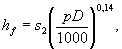 (P10.45)
but not less than 0.8s2.
The accepted
value of hf is specified in the process of calculating the
stress state of the flange in the cross-sections A-A, B-B,
C-C (see Fig. P10.2).
6.4.2. The moments
of resistance of the flange in the design cross-sections are calculated as
follows:
1) in the
cross-section A-A
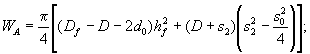 (P10.46)
2) in the cross-section
B-B
 (P10.47)
if y ≤ hf,
and
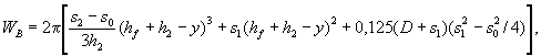 (P10.48)
if y > hf.
In the
formulas (P10.47) and (P10.48), the ordinate of the center of
gravity of the cross-section of the flange is calculated by the formula
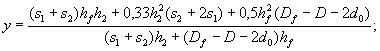 (P10.49)
3) in the
cross-section C-C
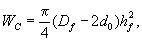 if hf
≤ s2. (P10.50)
if hf
≤ s2. (P10.50)
If hf
> s2, then the flange strength in the cross-section C-C
is assured and WC is not determined.
6.4.3. Strength
conditions in the design cross-sections A-A, B-B, C-C
are checked by the formula
σ
= max{M/WA;
M/WB; M/WC} ≤ [σ]. (P10.51)
If rated
stresses σ exceed permissible ones [σ], then the values of hf,
s2 and h2 shall be increased. Provided
that, it is necessary to increase the conicity i first.
The accepted
values of hf and s2 are recommended to be
increased in  times.
With the accepted flange dimensions, the calculations shall be repeated using
the formulas in items 4-6 of this Appendix until the values of the calculated
stresses are equal (with an error of no more than 5%) or less than the
permissible stresses.
times.
With the accepted flange dimensions, the calculations shall be repeated using
the formulas in items 4-6 of this Appendix until the values of the calculated
stresses are equal (with an error of no more than 5%) or less than the
permissible stresses.
6.5. When the
control of tightening the pins with the use of zero-torque force is not
provided, then on the basis of the maximum permissible force in the pins the
height of the face of flanges is determined by the formula
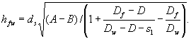 (P10.52)
If A ≤ B,
then the height of the flange face is equal to the value of hf,
obtained by the formulas in items 6.1, 6.2 and 6.4 of this
Appendix. Provided that, the auxiliary values of A for flanges with a
conical adapter and for flat flanges and B for flanges with a conical
adapter are determined by the formulas
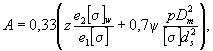 (P10.53)
where
 (P10.54)
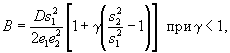 (P10.55)
where
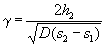 (P10.56)
and
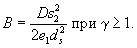 (P10.57)
For flat
flanges, the auxiliary value of B is found by the formula
 (P10.58)
To check the
height of the supporting clamp, use the formulas (P10.52), (P10.53)
and (P10.58), where it is necessary to replace e1 with
e6 and e2 with e5.
6.6. The final
flange height is selected by the highest value hf or hfw,
obtained by the formulas in items 6.1, 6.2, 6.4 and 6.5
of this Appendix.
If hfw
is assumed as the final flange height, then the calculation for the flange with
a conical adapter shall be repeated using the formulas in items 4, 5 and 6 of
this Appendix, proportionally increasing the values of s2 and
h2.
APPENDIX 11
RECOMMENDATIONS FOR DETERMINING THE
PROCESS INCREASE TO THE ELBOW WALL THICKNESS
1. The
recommendations of this Appendix can be used if there are no instructions in
the technical specifications for the manufacture of elbows for determining the
process increase.
2. In this Appendix,
the designations for the sizes of the elbows, shown in Fig. 4.5
hereof, are used. Formulas for determining wall thickness s, sR1,
sR2, sR3 are given in
item 4.2.2.3 hereof.
3. For bends
made on tube bending machinery by winding onto a sector, the process increase c12
is accepted only to the wall thickness sR1:
for pipes of heating
surfaces
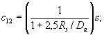
for other pipes
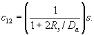
4. For stamped
elbows manufactured in closed dies, or bends made on machines with
high-frequency heating and axial preload, the process increase is assumed only
to the wall thickness sR1:
0.05s ≤ c12
≤ 0.1s.
5. For elbows,
made on horn-shaped cores, it is assumed with 12 = 0.
6. For
sectoral elbows, it is assumed c12 = 0.
7. For
stamp-welded elbows with two longitudinal welds located on the inner and outer
sides of the elbow, the process increase is assumed only to the wall thickness sR2:
0.05s ≤ c12
≤ 0.1s.
8. For
stamp-welded elbows with the location of the weld in the neutral zone of the
elbow, the process increase is assumed only to the wall thickness sR3:
0.05s ≤ c12
≤ 0.1s.
9. If the
determination of the c12 increase is carried out before the
final selection of the nominal wall thickness of the elbow, then it is
recommended that the nominal wall thickness of the elbow to be assumed as, for
example, the nominal wall thickness of the straight pipe, followed by
refinement of the final selected nominal wall thickness of the elbow.
APPENDIX 12
(recommended)
SIMPLIFIED CALCULATION FOR CYCLIC
STRENGTH
1. BASIC PROVISIONS
1.1. The
calculation method is applicable to the equipment and pipelines of groups B and
C.
1.2. The
calculation method is applicable to the equipment and pipelines in accordance
with item 1.1, satisfying the conditions of the following items.
1.3. The design
temperature of the walls of the equipment and pipelines does not exceed the
limits specified in Section 3.2 hereof for relevant materials.
1.4. Equipment
and pipelines meet the conditions of static strength and stability in
accordance with these Regulations.
1.5. The
calculation method does not apply to the case of imposing the high-frequency
loading from vibrations and pulsations of operating environment temperatures on
the low-frequency operational loading and is limited to cyclic loading with the
number of cycles of a given amplitude of not more than 106 during
operation.
2. DETERMINATION OF
CHANGE OF TEMPERATURES, STRESSES AND NUMBER OF OPERATING CYCLES
2.1. The
calculation is carried out for equipment and pipeline zones, where due to
stress concentrators (holes, changes in wall thickness, fillets, grooves,
threads, etc.), application of concentrated loads, edge effect, compounds of
steels with different elastic moduli E1T, E2T,
and expansion temperature coefficients α1T, α2T
and temperature difference, the increased cyclic local stresses occur.
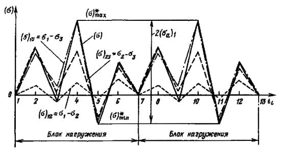
Fig. P12.1.
Graph of stress (σ) change
|
блок нагружения
|
loading unit
|
2.2. At the
first stage, a graph of the stress (σ) change is obtained using the dependences
(σ)ij, (σ)jk, (σ)ik for
the considered zone of the component of structure, obtained according to item 5.3.4
hereof (Fig. P12.1) for given loads and operating conditions.
2.3. Out of the
three dependences (σ)ij, (σ)jk, (σ)ik,
there is found the generalized dependence of successive half cycles of reduced
stresses, at the limiting points of which absolutely the highest (lowest)
stress values of the three above dependences are reached.
Generalized
dependency includes all the moments of time tl (1 ≤ l
≤ m), where at least one of the stresses (σ)ij, (σ)jk,
(σ)ik reaches the extreme value and has an extremum at each
of these moments (σ) = max{|(σ)ij|, |(σ)jk|,
|(σ)ik|} with the appropriate sign. In initial (l = 1)
and final (l = m) moments, the stress (σ) can take, inter alia,
values equal to zero.
2.4. From the
generalized dependence obtained according to item 2.3 of this Appendix,
a stress cycle with the largest amplitude is distinguished:
(σa)1 =
0.5[(σ)*max
- (σ)*min],
(P12.1)
where (σ)*max,
(σ)*min are algebraically largest and smallest given
stresses.
2.5. Other types
of cycles with smaller amplitudes of stresses (σa)i
are distinguished from the rest of the generalized dependence, guided by the
formula (P12.1), and 0.5 (m - 1) of types of cycles are obtained.
2.6. The
amplitude of the reduced local conditional elastic stress in the i-th
cycle is found by the formula
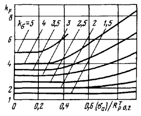
Fig. P12.2.
Coefficients of stress concentration
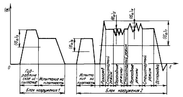
Fig. P12.3. Example
of drawing up blocks of loading and a graph of changes in the reduced stress in
the concentration zone (σ)
|
блок нагружения
|
loading unit
|
|
гидравлическое испытание
|
Hydrotest
|
|
испытание на плотность
|
Leak-tightness test
|
|
разогрев
|
Heating up
|
|
стационарный режим
|
Steady-state mode
|
|
переходные режимы
|
Transients
|
|
остановка
|
Shutdown
|
(σaF)
= KF,i(σa)i(φs)-1,
(P12.2)
where kF,I
is a stress concentration coefficient in the i-th cycle; φs
is a coefficient of reduction of the cyclic strength of a welded joint with
full weld penetration or a deposit welding.
In the absence
of data on values of φs, it can be assumed that φs
= 0.6, and in the absence of a weld φs = 1.
2.7.
Concentration coefficients KF,i are
determined by the formula
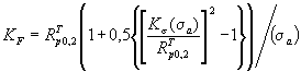 (P12.3)
or according to Fig. P12.2
depending on the relationship (σa)i/RTp0.2,
where RTp0.2 is a material yield
strength at a rated temperature; Kσ is a theoretical
coefficient of stress concentration determined from reference books and assumed
to be equal to the greatest value in the direction of circular and meridional
stresses in case of axial tension.
For metric
threads it is assumed that Kσ = 5. For incomplete-penetration
welded austenitic welds KF,i = 6.
Coefficient KF,i
to simplify the calculation, can be assumed the same for all types of cycles,
regardless of the amplitude value, and equal to its value for the type of cycle
with a maximum amplitude.
2.8. In the
absence of data according to item 2.3 of this Appendix, the dependence
of the reduced stresses can be obtained as follows.
2.8.1. The reduced
stresses (σ) in the considered zone are determined for physically feasible
loading blocks (Fig. P12.3) with the inclusion of operating modes of
loading, for example, for a vessel with a lid on threaded pins:
1) initial
condition, tightening of pins, hydraulic test, leak-tightness test, pressure
reduction to atmospheric pressure, initial condition;
2) initial
condition, tightening of pins, leak-tightness test, heating up, steady-state
mode, transients (for normal operation and abnormal operation), steady-state
mode, shutdown, pressure reduction to atmospheric pressure, initial condition.
2.8.2. Amplitude
of stress (σa)i of a half cycle in the i-th
transient or combination of modes is determined by the formula
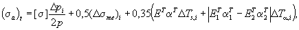 (P12.4)
where p is a
design pressure; ∆pi is a pressure change range in the
interval between time moments t1 and t2;
(∆σme)I is a change in the reduced stress caused
by a change in mechanical (compensatory) loads ∆Fmei in the
interval between time moments t1 and t2; ∆Ts,I
= |∆Ts,t1 - ∆Ts,t2|
is a difference of temperature differences across the wall thickness or mean
temperatures in two adjacent cross-sections of the component of structure
perpendicular to the mean surface in time moments t1 and t2;
∆Tα,i = |∆Tα,t1 - ∆Tα.t2|
is a difference of temperatures mean in wall thickness at the junction of
dissimilar steels with properties E1T, α1T
and E2T, α2T
in time moments t1 and t2.
Neighboring
cross-sections are those the distance between which is less than  , where Rs
is a mean value of radii of curvature in the middle of the wall thickness; s
is a mean wall thickness in adjacent points of the vessel, branch pipe, flange,
or other components.
, where Rs
is a mean value of radii of curvature in the middle of the wall thickness; s
is a mean wall thickness in adjacent points of the vessel, branch pipe, flange,
or other components.
Temperature
differences ∆Ts,i and ∆Tα,i,
range (∆σme)i, change ∆p are
determine at such moments of time of the i-th mode or combination of
modes when the reduced stress (σ) reaches extreme values. This shall consider
the signs of stress from pressure, mechanical loads and temperature differences
at the specified moments in time, otherwise the absolute values of stresses are
summed.
To obtain the
largest stress amplitudes, such combination of modes shall be considered, in
which changes in pressure, mechanical loads, temperatures cause minimum and
maximum stresses in the zone in question, for example, the effect of external
overpressure, and then internal heating, and then cooldown; alternating action
of mechanical loads. If any load does not change in the considered half-cycle,
then the corresponding values of ∆pi, ∆Fme,i,
∆Ts,i, ∆Tα,i in
the formula (P12.4) are assumed to be equal to zero. The obtained
dependence of the stress change in the block shall not have stress ruptures.
2.8.3. Temperature
difference ∆Tmax (°C) in the wall thickness s (m) of
material with the coefficients of thermal conductivity λ [W/(m2 ·
°C)] and thermal diffusivity a (m2/s) with one-sided heating
(cooling) by the working medium in the temperature range from T0
to Tk during the time tk (s) can be
determined by Fig. P12.4., where θ = s2/atk
is a dimensionless rate of temperature change of the medium; ∆θmax =
∆Tmax/(Tk - T0) is a
dimensionless temperature difference in the wall Bi = αs/λ is a
Biot number; α is a heat transfer coefficient, W/(m2 · °C).
Temperature
difference
∆Tmax = ∆θmax(Tk
– T0). (P12.5)
The time tmax
of reaching the maximum temperature difference ∆Tmax in the
wall can be determined using Fig. P12.5 by the formula
tmax = ∆Fomaxs2/a
+ tk, (P12.6)
where ∆Fomax
is a difference of the values of the Fourier criteria at moments of time tmax
and tk.
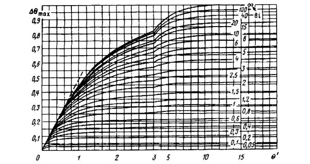
Fig. P12.4.
Dependencies for determining the maximum temperature difference in the wall
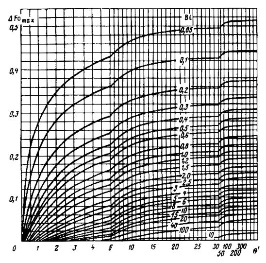
Fig. P12.5.
Dependencies for determining the time to reach the maximum temperature
difference in the wall
2.8.4. Amplitudes
of the reduced local conditional elastic stress (σaF)i
are found by the formula (P12.2) using instructions in items 2.4
- 2.7 of this Appendix.
2.8.5. In the
absence of data on the coefficients Kσ, amplitudes of
stresses (σaF)i in equipment and pipelines
can be determined by the formula
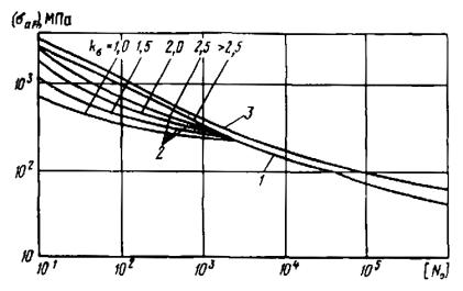
Fig. P12.6. Design
fatigue curves:
1 – for carbon, alloyed
(up to 360 °C) and austenitic (up to 450 °C) steels (RTm
≥ 400 MPa; zT ≥ 45 %; ET ≥ 180 GPa; RTp0.2/RTm
< 0.7); 1, 2 – for alloy steels at RTp0.2/RTm
≥ 0.7 (RTm ≥ 400 MPa; zT ≥ 45 %;
ET ≥ 195 GPa); 3 – for threaded components of alloyed
steel (up to 360 °C) (RTm ≥ 650 MPa; ET
≥ 195 GPa; zT ≥ 40 %)
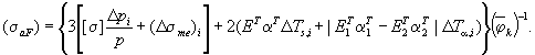 (P12.7)
All
instructions in the formula (P12.4) are applied to the formula (P12.7).
The formula (P12.7) is applicable for concentration zones and
full-penetration welds.
2.9. Set the
number of cycles Ni corresponding to each value of the
amplitude is set during the operation based on data on the repetition of modes
of operation and loading.
3. VERIFICATION OF CYCLIC STRENGTH
3.1. Cyclic
strength is checked by fatigue curves (Fig. P12.6).
At temperature
T, below the maximum value for the corresponding fatigue curve in Fig. P12.6,
the stress amplitude [σaF] when determining the number of
cycles shall be multiplied by the ratio Е360°C/ET
for carbon and alloy steels and Е450°C/ET –
for austenitic.
3.2. The
strength condition is checked by the formula
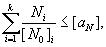 (P12.8)
where Ni
is a number of cycles of the i-th type during the operation; [N0]i
is a permissible number of cycles of the i-th type (is assumed according
to item 3.1); k is a total number of cycle types; [aN]
is an accumulated fatigue damage the limit value of which is equal to 0.4 for
equipment and pipelines of group B and 1.0 for group C.
Different
types of cycles are allowed to be combined and reduced to one design cycle. The
number of design cycles is equal to the sum of the numbers of combined cycles.
Permissible number of design cycles [N0] corresponds to the
maximum amplitude (σaF) from the combined types of cycles.
Types of
loading cycles with a stress amplitude lower than the stress amplitude along
the fatigue curve in Fig. P12.6 at [N0] = 106
are not considered if their number does not exceed 105.
Надписи на
рисунках:
|
МПа
|
MPa
|
|
кгс
|
kgf
|
|
м
|
m
|
|
мм
|
mm
|
|
ч
|
h
|
|
м/с2
|
m/s2
|
|
Гц
|
Hz
|
|
Н
|
N
|
|
или
|
or
|
|
где
|
where
|
|
кроме
|
except
|
|
при
|
at
|
|
если
|
if
|
|
при этом
|
here
|
|
а)
|
a)
|
|
б)
|
b)
|
|
в)
|
c)
|
|
г)
|
d)
|
|
д)
|
e)
|
|
е)
|
f)
|
|
ж)
|
g)
|
|
з)
|
h)
|
|
и)
|
i)
|
|
к)
|
j)
|
|
л)
|
k)
|